Generalized Additive Models#
Generalized Additive Models (GAMs) offer a powerful and flexible extension to traditional linear models by allowing for non-linear, additive relationships between each predictor and the outcome. Unlike standard linear regression, which assumes a strictly linear association between predictors and the response variable, GAMs replace each linear term with a smooth function, enabling the model to better capture complex patterns in the data. Thanks to their additive structure, each predictor contributes independently to the model, making it easy to interpret the effect of each variable.
So instead of using the standard linear function
we have something like this:
In short, instead of using fixed slope coefficients \(b_i\) that assume a straight-line relationship, we replace them with flexible (possibly non-linear) smooth functions \(f_i\) for each predictor. These functions can be anything from constant functions and polynomials to wavelets.
So in comparison to simple splines regression which (last semester) was introduced to predict \(y\) on the basis of a single predictor \(x\), GAMs are a generalization which allows us to predict \(y\) given multiple predictors \(x_1 ... x_p\).
Today’s data: The Diabetes dataset#
For today’s practical demonstration, we will work with the Diabetes dataset from scikit-learn. This dataset contains medical information collected from 442 diabetes patients, including:
Features: 10 baseline measures from the beginning of the study: age, sex, Body Mass Index (BMI), average blood pressure, as well as six blood serum measurements (e.g. cholesterol, blood sugar, etc.)
Target: A quantitative measure of disease progression one year after the baseline measurements were taken.
You can find more information here.
from sklearn import datasets
from sklearn.model_selection import train_test_split

# Get data
diabetes = datasets.load_diabetes(as_frame=True)
X = diabetes.data
y = diabetes.target

# Split the data into training and test set
X_train, X_test, y_train, y_test = train_test_split(X, y, test_size=0.3, random_state=42)
To explore the relationships between each feature and the target, we plot each predictor against the disease progression outcome. These scatter plots with simple linear regressions help us to visually assess whether the relationship between a feature and the target is linear or if we need a more flexible model approach:
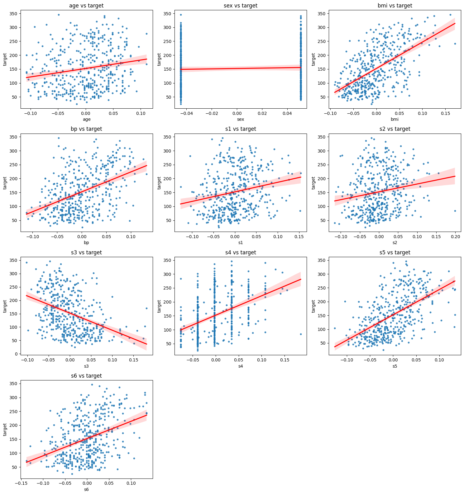
Although the linear regression fits seem to be reasonable, we might suspect that a more flexible approach could be beneficial, so let’s try it!
GAMs in Python#
There are multiple options for implementing GAMs. We will here use statsmodels, as you should already be familiar with it from the previouis semester. The workflow is the following:
Separate smooth (continuous) and categorical features
Create spline basis functions for the continuous features using B-splines
Fit the GAM with both the smooth and categorical predictors
from statsmodels.gam.api import GLMGam, BSplines

spline_features = ['age', 'bmi', 'bp', 's1', 's2', 's3', 's4', 's5', 's6']
categorical_features = ['sex']

# Create smoother for continuous variables
bs = BSplines(X_train[spline_features], df=[6]*len(spline_features), degree=[3]*len(spline_features))

# Fit GAM with smoother and exog for categorical
gam = GLMGam(y_train, exog=X_train[categorical_features], smoother=bs)
res = gam.fit()

print(res.summary())
                 Generalized Linear Model Regression Results
==============================================================================
Dep. Variable:                 target   No. Observations:                  309
Model:                         GLMGam   Df Residuals:                   263.00
Model Family:                Gaussian   Df Model:                        45.00
Link Function:               Identity   Scale:                          2998.6
Method:                         PIRLS   Log-Likelihood:                -1650.5
Date:                Mon, 27 Oct 2025   Deviance:                   7.8864e+05
Time:                        13:07:03   Pearson chi2:                 7.89e+05
No. Iterations:                     3   Pseudo R-squ. (CS):             0.7023
Covariance Type:            nonrobust
==============================================================================
                 coef    std err          z      P>|z|      [0.025      0.975]
------------------------------------------------------------------------------
sex         -289.6664     78.808     -3.676      0.000    -444.126    -135.206
age_s0       -32.4246     50.442     -0.643      0.520    -131.289      66.439
age_s1       -61.4878     28.887     -2.129      0.033    -118.105      -4.871
age_s2        -5.3132     39.461     -0.135      0.893     -82.655      72.029
age_s3       -42.6463     38.246     -1.115      0.265    -117.608      32.315
age_s4        18.0807     60.041      0.301      0.763     -99.598     135.759
bmi_s0        43.8396     54.386      0.806      0.420     -62.756     150.435
bmi_s1        19.4553     33.130      0.587      0.557     -45.479      84.390
bmi_s2        97.0613     48.512      2.001      0.045       1.980     192.142
bmi_s3        57.8888     49.412      1.172      0.241     -38.956     154.734
bmi_s4       252.4823     59.944      4.212      0.000     134.995     369.969
bp_s0         30.6097     58.249      0.525      0.599     -83.556     144.775
bp_s1         38.3179     38.098      1.006      0.315     -36.353     112.989
bp_s2         76.9274     49.565      1.552      0.121     -20.218     174.073
bp_s3         81.3546     48.055      1.693      0.090     -12.832     175.542
bp_s4        147.7945     57.513      2.570      0.010      35.070     260.519
s1_s0         58.6364    106.319      0.552      0.581    -149.744     267.017
s1_s1       -125.9137    154.677     -0.814      0.416    -429.075     177.247
s1_s2       -233.7171    336.444     -0.695      0.487    -893.135     425.701
s1_s3       -439.3612    450.331     -0.976      0.329   -1321.994     443.272
s1_s4       -351.3655    556.288     -0.632      0.528   -1441.670     738.939
s2_s0         26.6938     99.713      0.268      0.789    -168.741     222.128
s2_s1        125.9591    143.712      0.876      0.381    -155.712     407.630
s2_s2        274.4660    332.759      0.825      0.409    -377.729     926.661
s2_s3        464.5552    472.107      0.984      0.325    -460.758    1389.868
s2_s4        262.7111    613.544      0.428      0.669    -939.813    1465.235
s3_s0         14.3698     64.625      0.222      0.824    -112.292     141.032
s3_s1         40.7103     49.233      0.827      0.408     -55.784     137.205
s3_s2         39.5808     95.906      0.413      0.680    -148.392     227.554
s3_s3        101.7901    148.474      0.686      0.493    -189.214     392.794
s3_s4        120.5364    187.063      0.644      0.519    -246.101     487.174
s4_s0        -37.5731     46.372     -0.810      0.418    -128.461      53.315
s4_s1         11.2719     36.681      0.307      0.759     -60.622      83.166
s4_s2        -64.0818     65.922     -0.972      0.331    -193.286      65.123
s4_s3         48.0156     87.235      0.550      0.582    -122.961     218.992
s4_s4         25.2745    109.679      0.230      0.818    -189.693     240.242
s5_s0        -22.0863     49.386     -0.447      0.655    -118.882      74.709
s5_s1         26.4723     30.680      0.863      0.388     -33.660      86.605
s5_s2        127.4137     69.308      1.838      0.066      -8.428     263.255
s5_s3        174.7068    139.025      1.257      0.209     -97.776     447.190
s5_s4        264.2489    238.234      1.109      0.267    -202.681     731.179
s6_s0        -72.3705     79.891     -0.906      0.365    -228.954      84.213
s6_s1        -33.7499     51.643     -0.654      0.513    -134.969      67.469
s6_s2        -74.4075     61.859     -1.203      0.229    -195.648      46.833
s6_s3         -6.0775     59.770     -0.102      0.919    -123.224     111.069
s6_s4        -28.6995     62.161     -0.462      0.644    -150.532      93.133
==============================================================================
For the B-splines1 we choose:
df=[6]*len(spline_features)-> 6 basis functions per featuredegree=[3]*len(spline_features)-> cubic splines (degree 3)
The output includes parameter estimates for all spline basis functions and categorical variables:
The
coefcolumn shows the estimated effect.The
P>|z|column tells you whether the estimate is statistically significantThe Pseudo
R-squared (CS)gives a rough measure of model fit (here around 0.70)
Due to the additive nature of GAMs, we can isolate and visualise the effect of each smooth term individually. This helps us understand the relationship between each predictor and the response, controlling for all other variables:
import matplotlib.pyplot as plt
fig, ax = plt.subplots(3,3, figsize=(7,7))

for i, feature in enumerate(spline_features):
    res.plot_partial(i, cpr=True, ax=ax[i//3, i%3])
    ax[i//3, i%3].set_title(f"Partial Effect: {feature}")

plt.tight_layout()
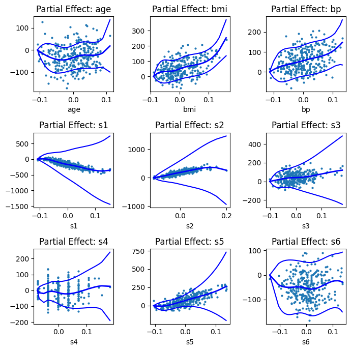
Each subplot shows how the modelled relationship between a feature and the target behaves nonlinearly. The cpr=True option adds confidence intervals around the estimated smooth curve.
Summary
GAMs allow flexible, interpretable models where you don’t assume linearity for every predictor.
statsmodelsmakes it easy to combine smooth terms (B-splines or alternatively Cyclic Cubic Splines) with categorical or linear predictors.You can inspect smooth effects with
.plot_partial(), and linear terms directly from the model summary.