Decision Trees#
Decision Trees are powerful and intuitive models used for both classification and regression problems. They work by recursively partitioning the feature space into smaller regions and assigning a prediction to each one. The tree structure is easy to interpret and visualise, making it a popular choice for understanding the relationship between inputs and outputs.
At their core, decision trees split the dataset into subsets based on feature values. Each split is chosen to maximise some purity measure, aiming to make the resulting subsets as homogeneous as possible.
Nodes: Points where decisions are made (internal nodes) or outcomes are assigned (leaf nodes).
Leaves (terminal nodes): Regions of the feature space with a predicted outcome.
Splits: Binary decisions on feature values, e.g., “is BMI ≤ 25?”.
The process is greedy and top-down, called recursive binary splitting.
Regression Trees#
The general usage of regression trees is identical to previous regression models:
from sklearn.tree import DecisionTreeRegressor

model = DecisionTreeRegressor()
model.fit()
As you learned in the lecture, there are a few additional parameters which we can choose, such as splitting criteria (where to split) or stopping criteria (when to stop splitting). You can look these up in the documentation. To see how these models perform, we can simply plot the predictions for two different models on synthetic data.
Generate data:
import numpy as np
from sklearn.model_selection import train_test_split

rng = np.random.RandomState(1)
X = np.sort(5 * rng.rand(100, 1), axis=0)
y = np.sin(X).ravel()
y[::5] += 3 * (0.5 - rng.rand(20))

X_train, X_test, y_train, y_test = train_test_split(X, y, test_size=0.3, random_state=0)
Fit two decision tree regressors to the data
from sklearn.tree import DecisionTreeRegressor

model1 = DecisionTreeRegressor(max_depth=2)
model2 = DecisionTreeRegressor(max_depth=6)

model1.fit(X_train, y_train)
model2.fit(X_train, y_train);
Plot the predictions to see how different models behave:
import matplotlib.pyplot as plt

X_range = np.arange(0.0, 5.0, 0.01)[:, np.newaxis]
pred1 = model1.predict(X_range)
pred2 = model2.predict(X_range);

plt.figure()
plt.scatter(X, y, s=30, c="darkorange", label="data")
plt.plot(X_range, pred1, color="cornflowerblue", label="max_depth=2", linewidth=2)
plt.plot(X_range, pred2, color="yellowgreen", label="max_depth=6", linewidth=2)
plt.xlabel("data")
plt.ylabel("target")
plt.title("Decision Tree Regression")
plt.legend();
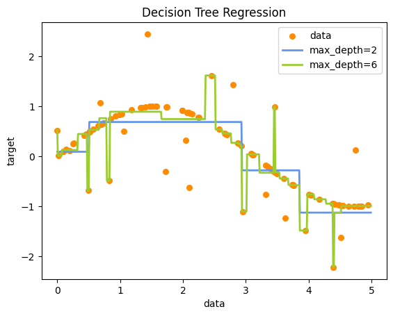
You can see that the max_depth=2 model is underfitting, while the max_depth=6 is overfitting. We can also can evaluate the models with usual performance metrics such as \(R^2\):
from sklearn.metrics import r2_score

r2_1 = r2_score(y_test, model1.predict(X_test))
r2_2 = r2_score(y_test, model2.predict(X_test))

print(f"R² (max_depth=2): {r2_1:.3f}")
print(f"R² (max_depth=6): {r2_2:.3f}")
R² (max_depth=2): 0.571
R² (max_depth=6): 0.472
Classification Trees#
The general usage of classification trees is identical to previous classification models:
import matplotlib.pyplot as plt
from sklearn.tree import DecisionTreeClassifier, plot_tree
from sklearn.datasets import load_iris

# Load data
iris = load_iris()
X, y = iris.data, iris.target

clf = DecisionTreeClassifier(max_depth=3)
clf.fit(X, y)

plt.figure(figsize=(12,8))
plot_tree(clf, feature_names=iris.feature_names, class_names=iris.target_names, filled=True, rounded=True, fontsize=14);
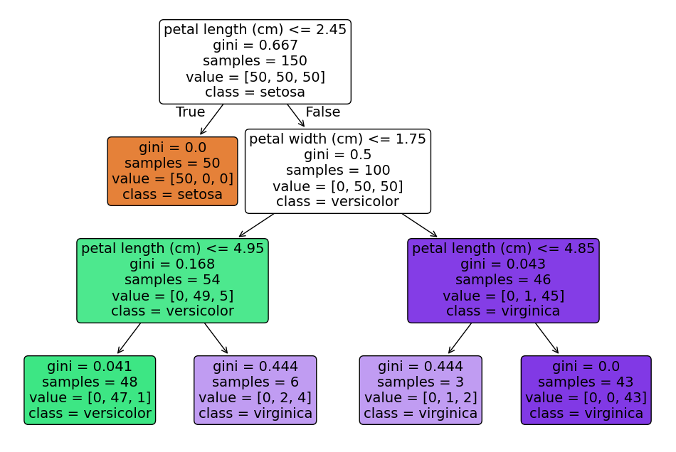
The tree plot of the fitted model contains the following information:
Decision nodes
These are the rectangles with a splitting criterion (e.g.
feature ≤ threshold)They represent the points where the model splits the data and asks “which branch next?”
Edges
The lines connecting nodes
Left edge follows the
truebranch (node condition met), right edge thefalsebranch
Leaf nodes
The terminal rectangles without further splits
The leaf nodes mark the final predicted class (
class)
Color fill
The shade corresponds to the majority class at that node
The epth of color indicates purity (dark = almost all one class; light = mixture)
Gini or entropy (implicitly encoded as the color fill)
Determines how “mixed” a node is when choosing splits
Pure nodes (all same class) are darkest with the color of the feature, impure nodes are white
Tree depth
The number of levels indicate how many successive decisions are made
Capped by the
max_depthparameter to control complexity
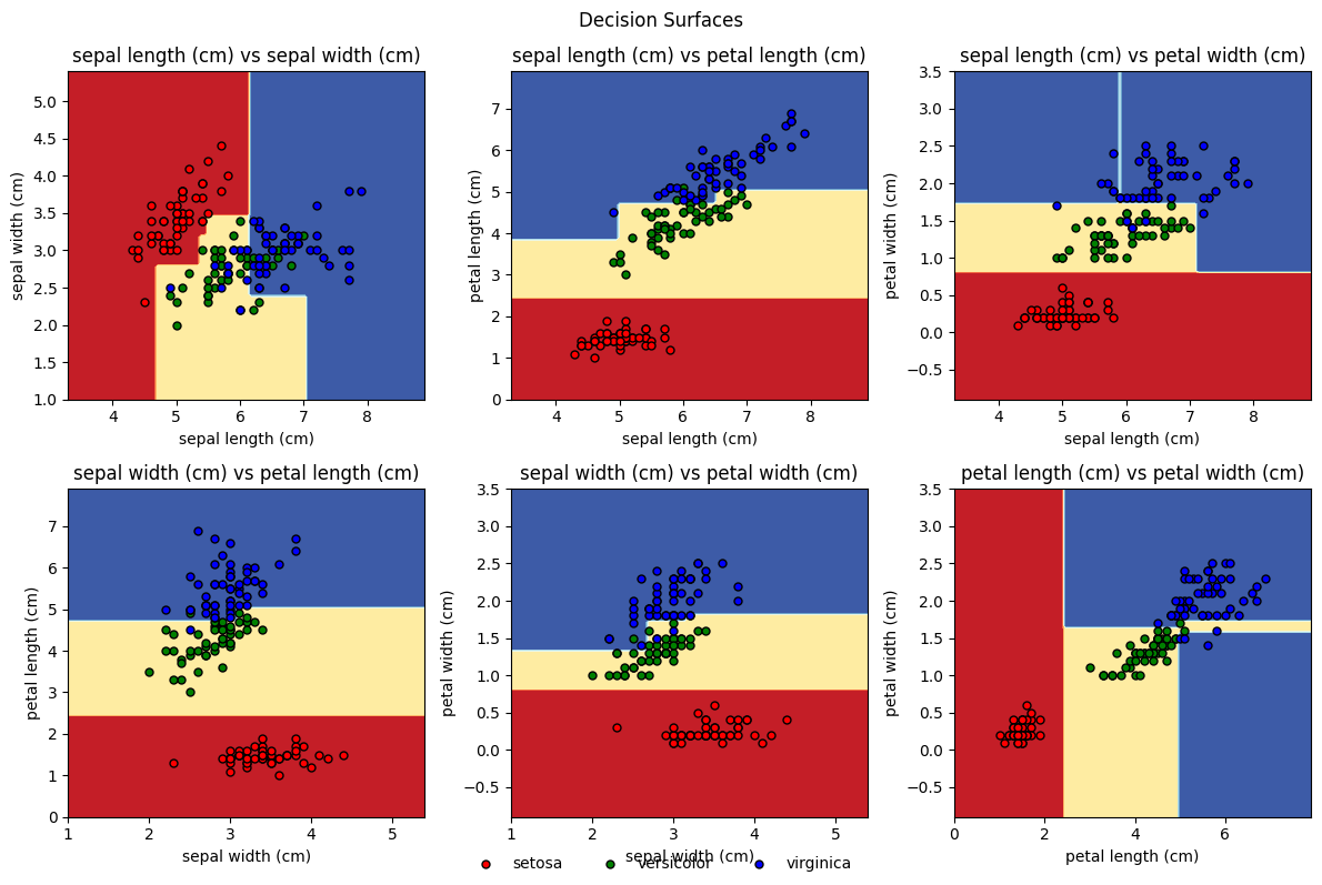
Another nice illustration is plotting the decision boundaries. As this works mostly with 2 features, we plot pairwise feature combinations:
Overfitting#
Large trees tend to overfit. To counter this we can do multiple things:
Prune the full-grown tree, also called bottom-up pruning or cost-complexity pruning (we saw this in the lecture)
Tune the hyperparameters that control the tree-growing behavior, also called top-down pruning.
Ensemble methods: bagging, random forests and boosting (will be introduced later)
Cost Complexity Pruning & Hyperparameter Tuning#
Cost complexity pruning means we add a penalty for tree size:
\(\text{Total Cost} = \text{RSS or Classification Error} + \alpha \cdot \text{Tree Size}\)
In scikit-learn this is controlled by ccp_alpha
ccp_alpha = 0-> no pruning -> full-grown treeccp_alpha > 0-> pruning -> smaller tree
We can further control the tree growing behaviour with hyperparameters such as
max_depthmin_samples_splitmin_samples_leaf
We can use a grid search to find the best combination for some of these hyperparameters:
import numpy as np
from sklearn.tree import DecisionTreeClassifier
from sklearn.model_selection import GridSearchCV

iris = load_iris()
X, y = iris.data, iris.target
X_train, X_test, y_train, y_test = train_test_split(X, y, test_size=0.3, random_state=0)

param_grid = {
    'ccp_alpha':         np.linspace(0.0, 0.2, 10),
    'max_depth':         [2, 4, 6, 8, 10, None],
    'min_samples_split': [2, 5, 10, 20],
    'min_samples_leaf':  [1, 2, 4, 8],
}

grid = GridSearchCV(DecisionTreeClassifier(), param_grid, cv=5)
grid.fit(X_train, y_train)

print("Best params:", grid.best_params_)
print("Test set accuracy:", grid.score(X_test, y_test))
Best params: {'ccp_alpha': np.float64(0.0), 'max_depth': 4, 'min_samples_leaf': 1, 'min_samples_split': 5}
Test set accuracy: 0.9777777777777777
Ensemble Methods#
Single trees have high variance. They are prone to overfitting and generally are not competetive when compared to more sophisticated models such als support vector machines. Ensemble methods try to solve these issues by combining many trees to reduce variance (bagging, random forest) or bias (boosting).
Bagging (Bootstrap Aggregation)#
Bagging involves the following steps:
Create multiple bootstrapped samples of the training set
Train a tree on each
Aggregate predictions
Classification: majority vote
Regression: average prediction
from sklearn.ensemble import BaggingClassifier
from sklearn.metrics import accuracy_score

bag = BaggingClassifier(n_estimators=100, random_state=0)
bag.fit(X_train, y_train)

accuracy_score(y_test, bag.predict(X_test))
0.9777777777777777
Random Forest#
Random Forest injects additional randomness by sub-sampling features at each split, further de-correlating the trees and improving variance reduction.
from sklearn.ensemble import RandomForestClassifier

rf = RandomForestClassifier(n_estimators=100, random_state=0)
rf.fit(X_train, y_train)

accuracy_score(y_test, rf.predict(X_test))
0.9777777777777777
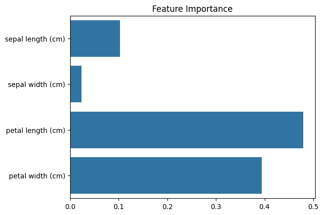
Feature importance can be visualised as:
import seaborn as sns

sns.barplot(x=rf.feature_importances_, y=iris.feature_names)
plt.title("Feature Importance");
Boosting#
Boosting builds trees sequentially. Each tree focuses on the residual errors of the previous one. Important parameters are:
n_estimators: number of treeslearning_rate: shrinkagmax_depth: tree depth
from xgboost import XGBClassifier

boost = XGBClassifier(n_estimators=100, learning_rate=0.1, max_depth=3)
boost.fit(X_train, y_train)
accuracy_score(y_test, boost.predict(X_test))
0.9777777777777777
Summary#
Summary
Method |
Description |
Pros |
Cons |
|---|---|---|---|
Decision Trees |
Split data via feature thresholds |
Highly interpretable, fast to train |
High variance → prone to overfitting |
Bagging |
Average many bootstrapped trees |
Reduces variance / overfitting |
Less interpretable; larger memory footprint |
Random Forest |
Bagging + random feature subsets at each split |
Further reduces variance; robust |
Slower to train and predict |
Boosting |
Sequentially fit to previous residuals / errors |
Low bias → often very accurate |
Can overfit noisy data; sensitive to hyperparameters |