5.1 Numpy

5.1 Numpy#

Before we begin, let’s pause for a second and try to think about which kind of data types and data structures structures we have learned about so far. Which ones can you remember? Do you think this is already enough for any kind of task you might want to achieve?

Solution

Python includes well known data types such as:

Integer numbers: 1,2,3, …
Floating point numbers: 1.2, 3.14, …
Strings: “Hello”
Boolean values: True/False
Empty value: None

The most important built-in data strucutures are:

Lists: [item1, item2, …]
Tuples: (item1, item2, …)
Dictionaries: {“key”: value(s)}

Arrays#

In fields like neuroscience, datasets can be large and often have more than two dimensions. For example, think of an fMRI scan composed of individual voxels (cubes) in three-dimensional space. And naturally, if you obtained more than one fMRI scan over time, you might have this as a fourth dimension. In such cases, n-dimensional arrays are a good way of storing and handling your data, as they do so as a single object. In any case, arrays are contiguious, meaning they have no “holes”, and they are homogenous, meaning they only consist of a single data type.

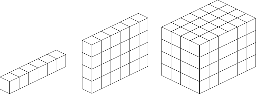
../../../_images/cubes.png — Fig. 4 N-dimensional arrays#

To work with arrays, we will use the NumPy library, which is the most important library for numerical and scientific computing in Python. Recall that by default, the Python namespace only includes a small number of built-in functions. So if we want to use functions that belong to numpy, we need to import it at the top of the script. In principle, you can chose any abbreviation you want (or none at all). However, it usually makes sense to stick to the conventions and import numpy as np.

import numpy as np

The core data structure of numpy are n-dimensional arrays called ndarray. We can create such an array from an existing list as follows:

my_list = [1,2,3,4]
my_array = np.array(my_list)

print(my_array)

[1 2 3 4]

While this might still look like a normal list on the surface, we can look at some additional attributes to see that it is, in fact, a numpy array:

print(f"Variable type: {type(my_array)}")
print(f"Data type:     {my_array.dtype}")
print(f"Data shape:    {my_array.shape}")

Variable type: <class 'numpy.ndarray'>
Data type:     int64
Data shape:    (4,)

You can see that the variable is now a <class 'numpy.ndarray'>. Type int64 means that the data stored in it are 64-bit integers and shape (4,) means that it is a one-dimensional array with 4 items. Similarly, we can create two-dimensional arrays from a list of lists:

list_of_lists = [[1,2,3], [7,8,9]]
my_array = np.array(list_of_lists)
print(my_array)
print(f"Shape: {my_array.shape}")

[[1 2 3]
 [7 8 9]]
Shape: (2, 3)

You can see that we created a two-dimensional array (you could also call it a matrix) of shape (2,3), meaning the array has two rows and three columns.

We can also create a new array from scratch and fill it with a specific value. Often, this is done by initializing an “empty” array containing only zeros:

my_array = np.zeros((4,5))
print(my_array)
print(f"Shape: {my_array.shape}")

[[0. 0. 0. 0. 0.]
 [0. 0. 0. 0. 0.]
 [0. 0. 0. 0. 0.]
 [0. 0. 0. 0. 0.]]
Shape: (4, 5)

However, in cases where 0 is a potential valid input, this can lead to hard to find errors. So an alternative would be to initialize an array filled with np.nan (“not a number”) values. Because if you then add e.g., a single value to it, it is more obvious that the other values are still missing:

my_array = np.full((4,5), np.nan)
my_array[1,2] = 1.0
print(my_array)
print(f"Shape: {my_array.shape}")

[[nan nan nan nan nan]
 [nan nan  1. nan nan]
 [nan nan nan nan nan]
 [nan nan nan nan nan]]
Shape: (4, 5)

Neuroimaging data#

Let’s look at some real data to get a better sense of why arrays are a useful thing to use. We use the nilearn package to load fMRI data of a single subject from the ADHD dataset and then convert the data into a numpy array with the nibabel package:

from nilearn import datasets
import nibabel as nib

haxby_dataset = datasets.fetch_adhd(n_subjects=1); # Download the Haxby dataset
fmri_img = nib.load(haxby_dataset.func[0]) # Load the fMRI data using nibabel
fmri_data = fmri_img.get_fdata() # Convert to a 4D numpy array
print(f"Shape of the fMRI data: {fmri_data.shape}")

[_add_readme_to_default_data_locations] Added README.md to /home/runner/nilearn_data
[get_dataset_dir] Dataset created in /home/runner/nilearn_data/adhd
[fetch_single_file] Downloading data from https://www.nitrc.org/frs/download.php/7781/adhd40_metadata.tgz ...

[fetch_single_file]  ...done. (0 seconds, 0 min)

[uncompress_file] Extracting data from /home/runner/nilearn_data/adhd/fbef5baff0b388a8c913a08e1d84e059/adhd40_metadata.tgz...
[uncompress_file] .. done.

[fetch_single_file] Downloading data from https://www.nitrc.org/frs/download.php/7782/adhd40_0010042.tgz ...

[_chunk_report_] 
Downloaded 17154048 of 44414948 bytes (38.6%%,    1.6s remaining)

[fetch_single_file]  ...done. (2 seconds, 0 min)

[uncompress_file] Extracting data from /home/runner/nilearn_data/adhd/e7ff5670bd594dcd9453e57b55d69dc9/adhd40_0010042.tgz...

[uncompress_file] .. done.

Shape of the fMRI data: (61, 73, 61, 176)

You can see that the data has shape (61, 73, 61, 176), meaning that it has four dimensions. fMRI data is similar to a picture which is composed of individual pixels, with the addition that the brain is a three-dimensional object and is thus separated in little cubes called voxels. As such three-dimensional scans are aquired in slices, the first two dimensions are the in-plane dimensions of the scan (\(61 * 73\) voxels), the third dimension are the \(61\) slices, and the third dimension is the time, telling us that \(176\) scans of the brain were obtained over time.

Indexing arrays#

We now know how to create arrays. But how can we can data in and out of them? Remember how we previously learned about indexing with lists. Indexing for arrays is fairly similar to this, however we have more flexibility in doing so. Let us first consider a one-dimensional array:

my_array = np.array([1,2,3,4,5])
print(my_array)
print(my_array[0])
print(my_array[3])
print(my_array[-1])
print(my_array[2:4])
print(my_array[:3])

[1 2 3 4 5]
1
4
5
[3 4]
[1 2 3]

We can see that all the indexing operations we pereviously learned about are still valid. my_array[0] gives us the value from the zeroth position, my_array[2] from the second position, and my_array[-1] from the last position. We can also apply slicing operations, whith my_array[2:4] giving us the second and the third position (remember that when slicing, the start is included, but the end is excluded), and my_array[:3] giving us all elements up to the second position.

Similarly, we can also index over two-dimensional arrays by separating the indices whithin the square brackets with commas:

my_array = np.array([[1,2,3],
                    [7,8,9]])
print(my_array)
print(my_array[0,0])
print(my_array[1,2])
print(my_array[:,0])
print(my_array[1,1:])

[[1 2 3]
 [7 8 9]]
1
9
[1 7]
[8 9]

Here, my_array[0,0] gives us the first item in the array, my_array[1,2] gives us the item at position two in the first row, my_array[:,0] gives us the entire first column and my_array[1,1:] gives us all items from the first row starting with the value at index 1.

Important

When indexing two-dimensional arrays, the first dimension always corresponds to the rows, and the second dimension corresponds to the columns!

So e.g. my_array[1,2] would give you the item in row 1, column 2. As a visualization, here are the individual indices for a a 2x3 array:

my_array	Column 0	Column 1	Column 2
Row 0	my_array[0,0]	my_array[0,1]	my_array[0,2]
Row 1	my_array[1,0]	my_array[1,1]	my_array[1,2]

Indexing whith conditionals#

An alternative way of indexing is to use logical oparations. This allows us to chose values from an array, only if they fulfil specific kind of conditions. For example, if we want to get all numbers in an array which are larger than 0, we can use the following expressions:

my_array = np.array([[0,2,0],
                    [0,8,9]])
larger_than_zero = my_array > 0
print(larger_than_zero)

[[False  True False]
 [False  True  True]]

You can see that the result are not yet the values which are larger than zero themselves, but a boolean array which tells us a which positions in the array our condition is Trueor False. We can then use this boolean array for indexing to extract the specific values from the array:

print(my_array[larger_than_zero])

[2 8 9]

This can be useful if you for example want to calculate some statistics over an array. For example, think about an array which holds reaction times measured in one of your experiments, and you want to exclude reaction times of more than one second from your analysis.

Arithmetic with arrays#

Another useful feature of arrays is that you can apply a variety of mathematical operations on them. For example, you can add and substract numbers from all elements in the array, or multiply/divide all elements in the array:

my_array = np.array([[1,2,3],
                     [4,5,6]])
print(my_array + 3)
print(my_array * 2)

[[4 5 6]
 [7 8 9]]
[[ 2  4  6]
 [ 8 10 12]]

Summary

The numpy library is the tool of choice when dealing with n-dimensional arrays in Python.