GLM#
Data preparation#
We will use the diabetes data set from the sklearn library for the following three exercises.
Loading the data
The code for loading the dataset is already provided. Look at the documentation of the
load_diabetes()function to familiarize yourself with the function and its outputs.Use the
DESCRattribute of the data set to get its description. Understand the variables, their meanings, and how they relate to the medical context (e.g., what each feature like BMI, age, and blood pressure represents in the context of diabetes).
Preparing the data
Rename the
targetcolumn of the todiabetesby using the.rename()method of the DataFrame. Search for its documentation if you are unsure how to use it.Print the DataFrame for visual inspection.
Hints:
If you’re using a local Python installation, you will need to install some packages:
pip install scikit-learn seaborn pingouin. Make sure to install them in thepsy111environmentIf you are using Goolge Colab, you only need to install the pingouin package by creating a code cell at the top of the script and writing:
!pip install pingouin.If you’re using a Jupyter Notebook, make sure to select any of “View as a scrollable element or open in a text editor” at the bottom of the output to see the entire description.
import pandas as pd
import seaborn as sns
import matplotlib.pyplot as plt
import statsmodels.formula.api as smf
import pingouin as pg
from sklearn import datasets
# 1. Load the data
diabetes = datasets.load_diabetes(as_frame=True)
diabetes_df = diabetes.frame
print(diabetes.DESCR)

# 2. Preparing the data
diabetes_df.rename(columns={'target': 'diabetes'}, inplace=True)
print(diabetes_df.head())
.. _diabetes_dataset:

Diabetes dataset
----------------

Ten baseline variables, age, sex, body mass index, average blood
pressure, and six blood serum measurements were obtained for each of n =
442 diabetes patients, as well as the response of interest, a
quantitative measure of disease progression one year after baseline.

**Data Set Characteristics:**

:Number of Instances: 442

:Number of Attributes: First 10 columns are numeric predictive values

:Target: Column 11 is a quantitative measure of disease progression one year after baseline

:Attribute Information:
    - age     age in years
    - sex
    - bmi     body mass index
    - bp      average blood pressure
    - s1      tc, total serum cholesterol
    - s2      ldl, low-density lipoproteins
    - s3      hdl, high-density lipoproteins
    - s4      tch, total cholesterol / HDL
    - s5      ltg, possibly log of serum triglycerides level
    - s6      glu, blood sugar level

Note: Each of these 10 feature variables have been mean centered and scaled by the standard deviation times the square root of `n_samples` (i.e. the sum of squares of each column totals 1).

Source URL:
https://www4.stat.ncsu.edu/~boos/var.select/diabetes.html

For more information see:
Bradley Efron, Trevor Hastie, Iain Johnstone and Robert Tibshirani (2004) "Least Angle Regression," Annals of Statistics (with discussion), 407-499.
(https://web.stanford.edu/~hastie/Papers/LARS/LeastAngle_2002.pdf)

        age       sex       bmi        bp        s1        s2        s3  \
0  0.038076  0.050680  0.061696  0.021872 -0.044223 -0.034821 -0.043401
1 -0.001882 -0.044642 -0.051474 -0.026328 -0.008449 -0.019163  0.074412
2  0.085299  0.050680  0.044451 -0.005670 -0.045599 -0.034194 -0.032356
3 -0.089063 -0.044642 -0.011595 -0.036656  0.012191  0.024991 -0.036038
4  0.005383 -0.044642 -0.036385  0.021872  0.003935  0.015596  0.008142

         s4        s5        s6  diabetes
0 -0.002592  0.019907 -0.017646     151.0
1 -0.039493 -0.068332 -0.092204      75.0
2 -0.002592  0.002861 -0.025930     141.0
3  0.034309  0.022688 -0.009362     206.0
4 -0.002592 -0.031988 -0.046641     135.0
Exercise 1: Multiple linear regression#
Estimate a multiple linear regression model using
bmi,bp, ands5to predict diabetes progression (diabetes).Estimate a second model with different predictors.
Compare the models. What is their R-squared value? What does it tell you about the performance of the models?
Tip: When working in Jupyter Notebooks, it might make sense to put different models/computations in separate code cells, so they can be evaluated individually and the outputs are easier to read.
model = smf.ols(formula='diabetes ~ bmi + bp + s5', data=diabetes_df)
results = model.fit()

print(results.summary())
                            OLS Regression Results
==============================================================================
Dep. Variable:               diabetes   R-squared:                       0.480
Model:                            OLS   Adj. R-squared:                  0.477
Method:                 Least Squares   F-statistic:                     134.8
Date:                Wed, 04 Dec 2024   Prob (F-statistic):           7.16e-62
Time:                        16:01:54   Log-Likelihood:                -2402.6
No. Observations:                 442   AIC:                             4813.
Df Residuals:                     438   BIC:                             4830.
Df Model:                           3
Covariance Type:            nonrobust
==============================================================================
                 coef    std err          t      P>|t|      [0.025      0.975]
------------------------------------------------------------------------------
Intercept    152.1335      2.653     57.342      0.000     146.919     157.348
bmi          603.0784     64.677      9.324      0.000     475.962     730.194
bp           262.2720     62.962      4.166      0.000     138.527     386.017
s5           543.8712     64.619      8.417      0.000     416.870     670.873
==============================================================================
Omnibus:                        9.591   Durbin-Watson:                   1.971
Prob(Omnibus):                  0.008   Jarque-Bera (JB):                6.859
Skew:                           0.183   Prob(JB):                       0.0324
Kurtosis:                       2.511   Cond. No.                         28.3
==============================================================================

Notes:
[1] Standard Errors assume that the covariance matrix of the errors is correctly specified.
model2 = smf.ols(formula='diabetes ~ sex + s1 + s6', data=diabetes_df)
results2 = model2.fit()

print(results2.summary())
                            OLS Regression Results
==============================================================================
Dep. Variable:               diabetes   R-squared:                       0.156
Model:                            OLS   Adj. R-squared:                  0.150
Method:                 Least Squares   F-statistic:                     26.99
Date:                Wed, 04 Dec 2024   Prob (F-statistic):           4.93e-16
Time:                        16:01:54   Log-Likelihood:                -2509.7
No. Observations:                 442   AIC:                             5027.
Df Residuals:                     438   BIC:                             5044.
Df Model:                           3
Covariance Type:            nonrobust
==============================================================================
                 coef    std err          t      P>|t|      [0.025      0.975]
------------------------------------------------------------------------------
Intercept    152.1335      3.380     45.006      0.000     145.490     158.777
sex          -56.5320     72.703     -0.778      0.437    -199.421      86.358
s1           156.3080     75.212      2.078      0.038       8.487     304.129
s6           580.0769     76.848      7.548      0.000     429.040     731.114
==============================================================================
Omnibus:                       32.093   Durbin-Watson:                   1.863
Prob(Omnibus):                  0.000   Jarque-Bera (JB):               17.955
Skew:                           0.335   Prob(JB):                     0.000126
Kurtosis:                       2.274   Cond. No.                         26.5
==============================================================================

Notes:
[1] Standard Errors assume that the covariance matrix of the errors is correctly specified.
Exercise 2: Correlations#
Correlations
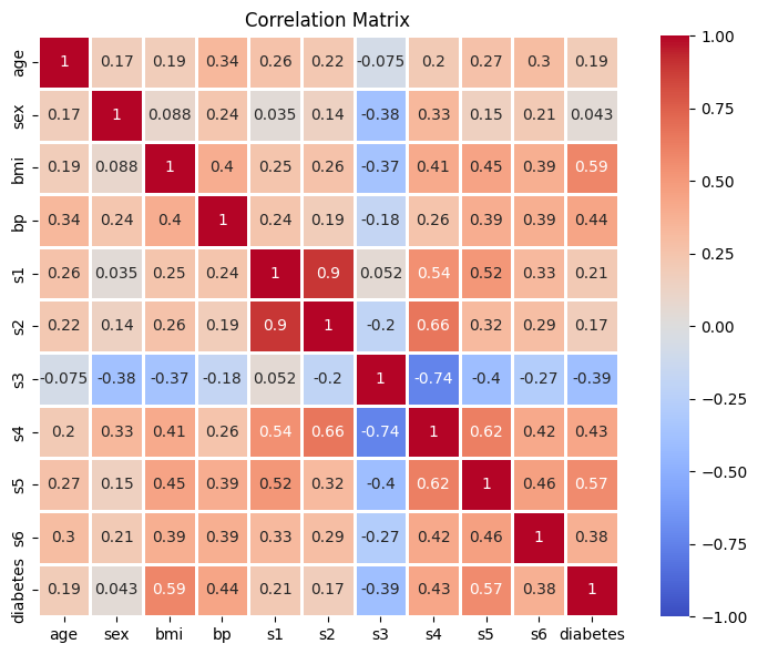
Compute the correlation matrix for all columns in the data
Print the shape of the correlation matrix. What shape does it have, and why?
Visualizing the data
Plot the correlation matrix by using
seaborn’sheatmap()function. The plot should have the following featurees:The cells in the plot should be annotated with the correlation values
The colormap should be
"coolwarm"(it’s a good choice for correlation values)The colorbar should range from
-1to1(because this is the full range correlation values can take)The cells in the plot should be quare (just because it looks nice)
The cells should be separated with lines of width
1(also because it looks nice)
Throug visual inspection, identify the variable that shows the highest correlation (positive or negative) with the target variable (diabetes progression)
# 1. Correlations
correlation_matrix = diabetes_df.corr()
print("Shape of the correlation matrix:", correlation_matrix.shape)

# 2. Visualizing the data
plt.figure(figsize=(8,6))
sns.heatmap(
    correlation_matrix,
    annot=True,
    cmap="coolwarm",
    vmin=-1,
    vmax=1,
    square=True,
    linewidths=1
)

plt.title('Correlation Matrix')
plt.tight_layout()
plt.show()
Shape of the correlation matrix: (11, 11)
Exercise 3: Partial Correlation#
Age could be influencing both BMI and diabetes progression. As people age, both their BMI and risk for diabetes may increase, potentially inflating the observed correlation between BMI and diabetes progression. By holding age constant, we can test whether the relationship between BMI and diabetes progression persists independently of age.
Hypothesis:
Null Hypothesis (\(H_0\)): There is no relationship between BMI and diabetes progression after controlling for age.
Alternative Hypothesis (\(H_1\)): There is a relationship between BMI and diabetes progression, even after controlling for age.
Tasks:
Use the
pingouinlibrary to calculate the partial correlation between BMI and diabetes progression, controlling for age.Compare the partial correlation coefficient to the original Pearson correlation coefficient. Did the correlation decrease after accounting for age? What does this suggest about age as a confounding factor?
partial_corr = pg.partial_corr(data=diabetes_df, x='bmi', y='diabetes', covar='age')
pearson_corr = diabetes_df['bmi'].corr(diabetes_df['diabetes'])

print(partial_corr)
print("\nNormal pearson correlation:", pearson_corr)

# Interpretation:
# After controlling for age, the relationship between BMI and diabetes progression persists, though it is slightly weaker.
# This suggests that while age has some influence, BMI remains a significant predictor of diabetes progression.
           n         r         CI95%         p-val
pearson  442  0.571553  [0.51, 0.63]  1.309246e-39

Normal pearson correlation: 0.5864501344746885
Voluntary exercise 1: Data wrangling#
We have previously loaded the diabetes dataset with the as_frame=True argument. If we do not specify this argument, the combined DataFrame will not be provided, but rather the data, target, and labels will be returned separately.
Familiarize yourself with the returns of the
load_diabetes()function.What kind of data types are the data, target, and labels?
Manually create the joint DataFrame by combining the data, target, and labels.
Verify that your operations were succesful (e.g. by printing the joint DataFrame).
Hint: There are multiple ways for creating a joint DataFrame. Have a look at section 5.2 if you need a refresher. You could, for example, join two DataFrames/Serier, or you could just add a new column to an existing DataFrame. Feel free to experiment! :)
# Voluntary exercise 1
dataset = datasets.load_diabetes()

# Get observations matrix (X) and target vector (y)
X, y, names = dataset.data, dataset.target, dataset.feature_names

# Option 1: Create a DataFrame and Series object from the numpy arrays and concatenate them
X_df= pd.DataFrame(X, columns=dataset.feature_names)
y_series = pd.Series(y, name="diabetes")
df1 = pd.concat([X_df, y_series], axis=1)
print(df1.head())
print("\n")

# Option 2: Create a DataFrame and append the diabetes column
df2= pd.DataFrame(X, columns=dataset.feature_names)
df2["diabetes"] = y
print(df2.head())
        age       sex       bmi        bp        s1        s2        s3  \
0  0.038076  0.050680  0.061696  0.021872 -0.044223 -0.034821 -0.043401
1 -0.001882 -0.044642 -0.051474 -0.026328 -0.008449 -0.019163  0.074412
2  0.085299  0.050680  0.044451 -0.005670 -0.045599 -0.034194 -0.032356
3 -0.089063 -0.044642 -0.011595 -0.036656  0.012191  0.024991 -0.036038
4  0.005383 -0.044642 -0.036385  0.021872  0.003935  0.015596  0.008142

         s4        s5        s6  diabetes
0 -0.002592  0.019907 -0.017646     151.0
1 -0.039493 -0.068332 -0.092204      75.0
2 -0.002592  0.002861 -0.025930     141.0
3  0.034309  0.022688 -0.009362     206.0
4 -0.002592 -0.031988 -0.046641     135.0