Polynomial Regression#
For the exercises we will use another mock-dataset. Assume the following scenario:
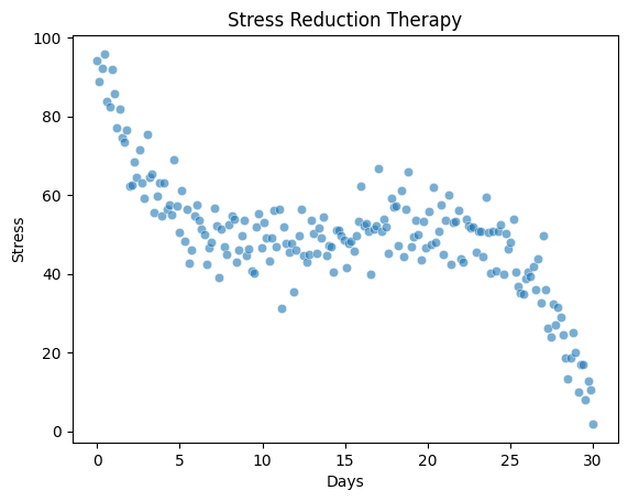
A research team tested a new therapy for reducing perceived stress over the course of 30 days. The generated data includes 200 stress level measures on a scale from 0 (no stress) to 100 (strong stress) at different time points after therapy start.
The data is stored in two columns:
days: The day of the measurement (0 to 30) after therapy startstress: The perceived stress level (0–100)
import numpy as np
import pandas as pd
import matplotlib.pyplot as plt
import seaborn as sns

# ----------------------------------------
# Simulate "Stress Reduction Therapy" Data
# ----------------------------------------
np.random.seed(42)

# Create data
n_points = 200
days = np.linspace(0, 30, n_points)
x_shifted = days - 15
true_stress = -((x_shifted**3) / 60 - x_shifted) + 50

# Add random noise and ensure scores between 0 and 100
noise = np.random.normal(0, 6.0, size=n_points)
stress = true_stress + noise
stress = np.clip(stress, 0, 100)

# Plot the data
fig, ax = plt.subplots()
sns.scatterplot(x=days, y=stress, alpha=0.6, ax=ax)
ax.set(xlabel='Days', ylabel='Stress', title='Stress Reduction Therapy');
Exercise 1: Fitting a linear model#
Please fit a simple linear regression model to predict stress based on days. Please use the syntax as introduced in the previous chapters using PolynomialFeatures so it will be easy to explore higher-order models later.
You tasks are:
Create features for a linear regression using
PolynomialFeaturesFit a linear model
Print and discuss the model summary
Plot the regression line on top of the data
Create a second plot for the residuals (either as a subplot or as two separate plots). Answer the following questions:
Are there patterns in the residuals that suggest the model is missing curvature?
Does the residual plot show systematic deviations (e.g., stress is consistently under/over-predicted at certain times)?
import statsmodels.api as sm
from sklearn.preprocessing import PolynomialFeatures

# Create features
features = PolynomialFeatures(degree=1, include_bias=True)
features_p1 = features.fit_transform(days.reshape(-1, 1))

# Fit the model
model = sm.OLS(stress, features_p1)
model_fit = model.fit()
predictions = model_fit.predict(features_p1)
residuals = model_fit.resid

# Print model summary
print(model_fit.summary())

# Plot the data
fig, ax = plt.subplots(1,2, figsize=(8, 4))

sns.scatterplot(x=days, y=stress, alpha=0.6, ax=ax[0])
ax[0].plot(days, predictions, color='red')
ax[0].set(xlabel='Time (days)', ylabel='Stress Score', title="Linear Model")
ax[1].plot(days, residuals, color='green', alpha = 0.6, linestyle='', marker='*') # Alternatively you can use sns.scatterplot() as previous sections or ax.scatter() as in Ex.2 solutions
ax[1].set(xlabel='Time (days)', ylabel='Residuals', title="Residuals")
ax[1].axhline(0, linestyle='--');
                            OLS Regression Results
==============================================================================
Dep. Variable:                      y   R-squared:                       0.501
Model:                            OLS   Adj. R-squared:                  0.499
Method:                 Least Squares   F-statistic:                     198.9
Date:                Wed, 22 Jan 2025   Prob (F-statistic):           1.01e-31
Time:                        11:35:15   Log-Likelihood:                -757.00
No. Observations:                 200   AIC:                             1518.
Df Residuals:                     198   BIC:                             1525.
Df Model:                           1
Covariance Type:            nonrobust
==============================================================================
                 coef    std err          t      P>|t|      [0.025      0.975]
------------------------------------------------------------------------------
const         68.1594      1.509     45.173      0.000      65.184      71.135
x1            -1.2269      0.087    -14.102      0.000      -1.399      -1.055
==============================================================================
Omnibus:                        0.372   Durbin-Watson:                   0.577
Prob(Omnibus):                  0.830   Jarque-Bera (JB):                0.495
Skew:                           0.088   Prob(JB):                        0.781
Kurtosis:                       2.831   Cond. No.                         34.6
==============================================================================

Notes:
[1] Standard Errors assume that the covariance matrix of the errors is correctly specified.
Exercise 2: Improving the model#
Do you think the linear model from the previous exercise can be improved? Which kind of polynomial might be suitable for the present data? Copy your code from the previous exercise and explore polynomials of different orders.
# Create features
features = PolynomialFeatures(degree=3, include_bias=True)
features_p1 = features.fit_transform(days.reshape(-1, 1))

# Fit the model
model = sm.OLS(stress, features_p1)
model_fit = model.fit()
predictions = model_fit.predict(features_p1)
residuals = model_fit.resid

# Print model summary
print(model_fit.summary())

# Plot the data
fig, ax = plt.subplots(1,2, figsize=(8, 4))

ax[0].scatter(days, stress, color='blue', alpha=0.4, marker='o', s=38) # Alternatively you can use sns.scatterplot() as you saw in previous sections
ax[0].plot(days, predictions, color='red')
ax[0].set(xlabel='Time (days)', ylabel='Stress Score', title="Cubic Model")
ax[1].scatter(days, residuals, color='green', alpha=0.4 ,linestyle='', marker='*')
ax[1].set(xlabel='Time (days)', ylabel='Residuals', title="Residuals")
ax[1].axhline(0, linestyle='--')
ax[1].set_ylim(-30, 30);
                            OLS Regression Results
==============================================================================
Dep. Variable:                      y   R-squared:                       0.865
Model:                            OLS   Adj. R-squared:                  0.863
Method:                 Least Squares   F-statistic:                     419.7
Date:                Wed, 22 Jan 2025   Prob (F-statistic):           4.93e-85
Time:                        11:35:15   Log-Likelihood:                -626.06
No. Observations:                 200   AIC:                             1260.
Df Residuals:                     196   BIC:                             1273.
Df Model:                           3
Covariance Type:            nonrobust
==============================================================================
                 coef    std err          t      P>|t|      [0.025      0.975]
------------------------------------------------------------------------------
const         91.2567      1.553     58.776      0.000      88.195      94.319
x1           -10.6397      0.449    -23.679      0.000     -11.526      -9.754
x2             0.7892      0.035     22.642      0.000       0.720       0.858
x3            -0.0176      0.001    -23.020      0.000      -0.019      -0.016
==============================================================================
Omnibus:                        0.493   Durbin-Watson:                   2.121
Prob(Omnibus):                  0.782   Jarque-Bera (JB):                0.515
Skew:                           0.118   Prob(JB):                        0.773
Kurtosis:                       2.922   Cond. No.                     4.16e+04
==============================================================================

Notes:
[1] Standard Errors assume that the covariance matrix of the errors is correctly specified.
[2] The condition number is large, 4.16e+04. This might indicate that there are
strong multicollinearity or other numerical problems.
Voluntary exercise: Centering predictors#
Please center the TimeDays predictor and then fit a cubic model to the data. Print the model summary and discuss how the interpretation of the coefficients changes. Do you think it makes sense to center the predictr in this example?
# Center the days
days_centered = days - np.mean(days)

# Create features
features = PolynomialFeatures(degree=3, include_bias=True)
features_p1 = features.fit_transform(days_centered.reshape(-1, 1))

# Fit the model
model = sm.OLS(stress, features_p1)
model_fit = model.fit()
predictions = model_fit.predict(features_p1)
residuals = model_fit.resid

# Print model summary
print(model_fit.summary())

# Plot the data
fig, ax = plt.subplots(1,2, figsize=(8, 4))

ax[0].scatter(days_centered, stress, color='blue', alpha=0.4, marker='o', s=38) # Alternatively you can use sns.scatterplot() as you saw in previous sections
ax[0].plot(days_centered, predictions, color='red')
ax[0].set(xlabel='Time (days)', ylabel='Stress Score', title="Cubic Model")
ax[1].scatter(days_centered, residuals, color='green', alpha=0.4 ,linestyle='', marker='*')
ax[1].set(xlabel='Time (days)', ylabel='Residuals', title="Residuals")
ax[1].axhline(0, linestyle='--')
ax[1].set_ylim(-30, 30);
                            OLS Regression Results
==============================================================================
Dep. Variable:                      y   R-squared:                       0.865
Model:                            OLS   Adj. R-squared:                  0.863
Method:                 Least Squares   F-statistic:                     419.7
Date:                Wed, 22 Jan 2025   Prob (F-statistic):           4.93e-85
Time:                        17:04:51   Log-Likelihood:                -626.06
No. Observations:                 200   AIC:                             1260.
Df Residuals:                     196   BIC:                             1273.
Df Model:                           3
Covariance Type:            nonrobust
==============================================================================
                 coef    std err          t      P>|t|      [0.025      0.975]
------------------------------------------------------------------------------
const         49.8956      0.593     84.113      0.000      48.726      51.065
x1             1.1698      0.114     10.298      0.000       0.946       1.394
x2            -0.0019      0.006     -0.317      0.751      -0.013       0.010
x3            -0.0176      0.001    -23.020      0.000      -0.019      -0.016
==============================================================================
Omnibus:                        0.493   Durbin-Watson:                   2.121
Prob(Omnibus):                  0.782   Jarque-Bera (JB):                0.515
Skew:                           0.118   Prob(JB):                        0.773
Kurtosis:                       2.922   Cond. No.                     1.94e+03
==============================================================================

Notes:
[1] Standard Errors assume that the covariance matrix of the errors is correctly specified.
[2] The condition number is large, 1.94e+03. This might indicate that there are
strong multicollinearity or other numerical problems.

Voluntary exercise 2: Data handling#
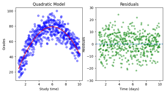
Now study the structure of study_time_p2. Instead of using the package from sklearn.preprocessing, PolynomialFeatures, find a way to manually create a matrix of shape (500, 3) with the same information as study_time_p2. Fit the new model using your manual_study_time_p2 and plot it in a new subplot next to the previous model. Are the two model comparable? Did anything change?
# ----------------------------------------
# Simulate "Study-grade" Data
# ----------------------------------------
np.random.seed(69)
study_time = np.linspace(1, 10, 500)
h = 6
k = 80
grades = -(k / (h**2)) * (study_time - h)**2 + k + np.random.normal(0, 8, study_time.shape)
grades = np.clip(grades, 0, 100) # ensure we only have grades between 0 and 100

# Create a DataFrame
df = pd.DataFrame({"study_time": study_time, "grades": grades})

# Create feature variable to be studied and replicated
polynomial_features_p2 = PolynomialFeatures(degree=2, include_bias=True)
study_time_p2 = polynomial_features_p2.fit_transform(study_time.reshape(-1, 1))
print(study_time_p2)
print(study_time_p2.shape)

# Create quadratic features
biases             = np.ones(500)
study_time_squared = study_time*study_time
manual_study_time_p2 = np.vstack([biases, study_time, study_time_squared])
manual_study_time_p2 = manual_study_time_p2.T
print(f"Shape of our biases: {biases.shape}")
print(f"Shape of our x squared: {study_time_squared.shape}")
print(f"Shape of our variable containing second degree features: {manual_study_time_p2.shape}")

# Fit the model
model = sm.OLS(grades, manual_study_time_p2)
model_fit = model.fit()
predictions = model_fit.predict(manual_study_time_p2)
residuals = model_fit.resid

# Print model summary
print(model_fit.summary())

# Plot the data
fig, ax = plt.subplots(1,2, figsize=(8, 4))

ax[0].scatter(study_time, grades, color='blue', alpha=0.4, marker='o', s=38) # Alternatively you can use sns.scatterplot() as you saw in previous sections
ax[0].plot(study_time, predictions, color='red')
ax[0].set(xlabel='Study time)', ylabel='Grades', title="Quadratic Model")
ax[1].scatter(study_time, residuals, color='green', alpha=0.4 ,linestyle='', marker='*')
ax[1].set(xlabel='Time (days)', ylabel='Residuals', title="Residuals")
ax[1].axhline(0, linestyle='--')
ax[1].set_ylim(-30, 30);
[[  1.           1.           1.        ]
 [  1.           1.01803607   1.03639744]
 [  1.           1.03607214   1.07344549]
 ...
 [  1.           9.96392786  99.27985831]
 [  1.           9.98196393  99.63960386]
 [  1.          10.         100.        ]]
(500, 3)
Shape of our biases: (500,)
Shape of our x squared: (500,)
Shape of our variable containing second degree features: (500, 3)
                            OLS Regression Results
==============================================================================
Dep. Variable:                      y   R-squared:                       0.750
Model:                            OLS   Adj. R-squared:                  0.749
Method:                 Least Squares   F-statistic:                     744.5
Date:                Wed, 22 Jan 2025   Prob (F-statistic):          3.14e-150
Time:                        17:04:54   Log-Likelihood:                -1771.1
No. Observations:                 500   AIC:                             3548.
Df Residuals:                     497   BIC:                             3561.
Df Model:                           2
Covariance Type:            nonrobust
==============================================================================
                 coef    std err          t      P>|t|      [0.025      0.975]
------------------------------------------------------------------------------
const          0.2520      1.696      0.149      0.882      -3.080       3.584
x1            26.3391      0.695     37.874      0.000      24.973      27.705
x2            -2.1972      0.062    -35.524      0.000      -2.319      -2.076
==============================================================================
Omnibus:                        4.382   Durbin-Watson:                   2.014
Prob(Omnibus):                  0.112   Jarque-Bera (JB):                3.932
Skew:                          -0.149   Prob(JB):                        0.140
Kurtosis:                       2.685   Cond. No.                         231.
==============================================================================

Notes:
[1] Standard Errors assume that the covariance matrix of the errors is correctly specified.