Spline Regression#
For the exercises, we will continue with the same data as in the previous sections. Again, we want to predict wage from age in the Mid-Atlantic Wage Dataset.
# Uncomment the following line when working in Colab
# !pip install ISLP
import numpy as np
import matplotlib.pyplot as plt
import seaborn as sns
import patsy
import statsmodels.api as sm
from ISLP import load_data

df = load_data('Wage')
print(df.head())
   year  age            maritl      race        education              region  \
0  2006   18  1. Never Married  1. White     1. < HS Grad  2. Middle Atlantic
1  2004   24  1. Never Married  1. White  4. College Grad  2. Middle Atlantic
2  2003   45        2. Married  1. White  3. Some College  2. Middle Atlantic
3  2003   43        2. Married  3. Asian  4. College Grad  2. Middle Atlantic
4  2005   50       4. Divorced  1. White       2. HS Grad  2. Middle Atlantic

         jobclass          health health_ins   logwage        wage
0   1. Industrial       1. <=Good      2. No  4.318063   75.043154
1  2. Information  2. >=Very Good      2. No  4.255273   70.476020
2   1. Industrial       1. <=Good     1. Yes  4.875061  130.982177
3  2. Information  2. >=Very Good     1. Yes  5.041393  154.685293
4  2. Information       1. <=Good     1. Yes  4.318063   75.043154
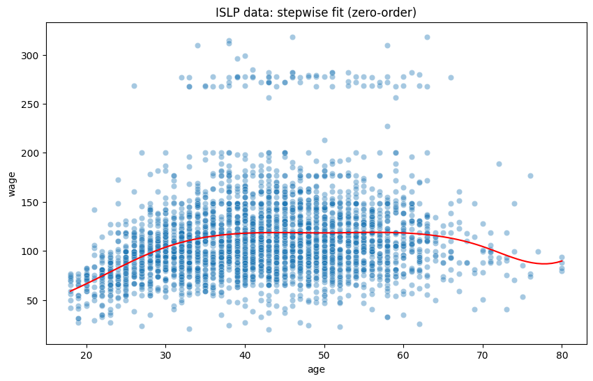
Exercise 1: Custom cut points#
Create a regression model to predict
wagefromageby using stepwise functions. However, instead of separating the data into 4 evenly sized bins, this time create custom cut points at age 30, 40, 50, 60, and 70.Print and interpret the model summary
Plot the model
# Fit the model with custom knots
transformed_age = patsy.dmatrix("bs(age, knots=(30,40,50,60,70), degree=0)",
                                data={"age": df['age']},
                                return_type='dataframe')

model = sm.OLS(df['wage'], transformed_age)
model_fit = model.fit()

print(model_fit.summary())

# Plot the model
plt.figure(figsize=(10, 6))
xp = np.linspace(df['age'].min(), df['age'].max(), 100)
xp_trans = patsy.dmatrix("bs(xp, knots=(30,40,50,60,70), degree=0)",
                         data={"xp": xp},
                         return_type='dataframe')

predictions = model_fit.predict(xp_trans)

sns.scatterplot(data=df, x="age", y="wage", alpha=0.4)
plt.plot(xp, predictions, color='red')
plt.title("ISLP data: stepwise fit (zero-order)");
                            OLS Regression Results
==============================================================================
Dep. Variable:                   wage   R-squared:                       0.070
Model:                            OLS   Adj. R-squared:                  0.068
Method:                 Least Squares   F-statistic:                     44.90
Date:                Wed, 22 Jan 2025   Prob (F-statistic):           7.91e-45
Time:                        11:38:41   Log-Likelihood:                -15341.
No. Observations:                3000   AIC:                         3.069e+04
Df Residuals:                    2994   BIC:                         3.073e+04
Df Model:                           5
Covariance Type:            nonrobust
====================================================================================================================
                                                       coef    std err          t      P>|t|      [0.025      0.975]
--------------------------------------------------------------------------------------------------------------------
Intercept                                           86.7282      1.903     45.573      0.000      82.997      90.460
bs(age, knots=(30, 40, 50, 60, 70), degree=0)[0]    25.3694      2.395     10.594      0.000      20.674      30.065
bs(age, knots=(30, 40, 50, 60, 70), degree=0)[1]    32.2987      2.315     13.950      0.000      27.759      36.838
bs(age, knots=(30, 40, 50, 60, 70), degree=0)[2]    30.5690      2.481     12.324      0.000      25.705      35.433
bs(age, knots=(30, 40, 50, 60, 70), degree=0)[3]    30.8021      3.591      8.578      0.000      23.762      37.843
bs(age, knots=(30, 40, 50, 60, 70), degree=0)[4]     9.2232      7.070      1.305      0.192      -4.639      23.085
==============================================================================
Omnibus:                     1081.976   Durbin-Watson:                   1.965
Prob(Omnibus):                  0.000   Jarque-Bera (JB):             4742.790
Skew:                           1.707   Prob(JB):                         0.00
Kurtosis:                       8.128   Cond. No.                         10.9
==============================================================================

Notes:
[1] Standard Errors assume that the covariance matrix of the errors is correctly specified.

Exercise 2: Higher-order splines#
Please fit and plot a second-order spline regression model with cut points at age 30, 50, and 70
Please fit and plot a third-order spline regression model with cut points at age 30, 50, and 70. Discuss the differences between the models. Does the third-order term significantly improve the model?
# Fit the model with custom knots
transformed_age = patsy.dmatrix("bs(age, knots=(30,50,70), degree=2)",
                                data={"age": df['age']},
                                return_type='dataframe')

model = sm.OLS(df['wage'], transformed_age)
model_fit = model.fit()

print(model_fit.summary())

# Plot the model
plt.figure(figsize=(10, 6))
xp = np.linspace(df['age'].min(), df['age'].max(), 100)
xp_trans = patsy.dmatrix("bs(xp, knots=(30,50,70), degree=2)",
                         data={"xp": xp},
                         return_type='dataframe')

predictions = model_fit.predict(xp_trans)

sns.scatterplot(data=df, x="age", y="wage", alpha=0.4)
plt.plot(xp, predictions, color='red')
plt.title("ISLP data: stepwise fit (zero-order)");
                            OLS Regression Results
==============================================================================
Dep. Variable:                   wage   R-squared:                       0.086
Model:                            OLS   Adj. R-squared:                  0.084
Method:                 Least Squares   F-statistic:                     56.07
Date:                Wed, 22 Jan 2025   Prob (F-statistic):           7.09e-56
Time:                        11:38:42   Log-Likelihood:                -15316.
No. Observations:                3000   AIC:                         3.064e+04
Df Residuals:                    2994   BIC:                         3.068e+04
Df Model:                           5
Covariance Type:            nonrobust
============================================================================================================
                                               coef    std err          t      P>|t|      [0.025      0.975]
------------------------------------------------------------------------------------------------------------
Intercept                                   53.6414      6.086      8.813      0.000      41.708      65.575
bs(age, knots=(30, 50, 70), degree=2)[0]    37.4841      7.890      4.751      0.000      22.014      52.954
bs(age, knots=(30, 50, 70), degree=2)[1]    69.6654      5.983     11.644      0.000      57.935      81.396
bs(age, knots=(30, 50, 70), degree=2)[2]    63.2010      7.146      8.844      0.000      49.189      77.213
bs(age, knots=(30, 50, 70), degree=2)[3]    50.1480     10.036      4.997      0.000      30.470      69.826
bs(age, knots=(30, 50, 70), degree=2)[4]    30.9407     19.443      1.591      0.112      -7.183      69.064
==============================================================================
Omnibus:                     1098.635   Durbin-Watson:                   1.961
Prob(Omnibus):                  0.000   Jarque-Bera (JB):             4981.584
Skew:                           1.723   Prob(JB):                         0.00
Kurtosis:                       8.290   Cond. No.                         32.0
==============================================================================

Notes:
[1] Standard Errors assume that the covariance matrix of the errors is correctly specified.

# Fit the model with custom knots
transformed_age = patsy.dmatrix("bs(age, knots=(30,50,70), degree=3)",
                                data={"age": df['age']},
                                return_type='dataframe')

model = sm.OLS(df['wage'], transformed_age)
model_fit = model.fit()

print(model_fit.summary())

# Plot the model
plt.figure(figsize=(10, 6))
xp = np.linspace(df['age'].min(), df['age'].max(), 100)
xp_trans = patsy.dmatrix("bs(xp, knots=(30,50,70), degree=3)",
                         data={"xp": xp},
                         return_type='dataframe')

predictions = model_fit.predict(xp_trans)

sns.scatterplot(data=df, x="age", y="wage", alpha=0.4)
plt.plot(xp, predictions, color='red')
plt.title("ISLP data: stepwise fit (zero-order)");
                            OLS Regression Results
==============================================================================
Dep. Variable:                   wage   R-squared:                       0.087
Model:                            OLS   Adj. R-squared:                  0.086
Method:                 Least Squares   F-statistic:                     47.77
Date:                Wed, 22 Jan 2025   Prob (F-statistic):           3.20e-56
Time:                        11:38:42   Log-Likelihood:                -15313.
No. Observations:                3000   AIC:                         3.064e+04
Df Residuals:                    2993   BIC:                         3.068e+04
Df Model:                           6
Covariance Type:            nonrobust
============================================================================================================
                                               coef    std err          t      P>|t|      [0.025      0.975]
------------------------------------------------------------------------------------------------------------
Intercept                                   58.9573      7.672      7.685      0.000      43.915      73.999
bs(age, knots=(30, 50, 70), degree=3)[0]    14.1773     10.772      1.316      0.188      -6.944      35.299
bs(age, knots=(30, 50, 70), degree=3)[1]    65.9159      7.649      8.618      0.000      50.918      80.914
bs(age, knots=(30, 50, 70), degree=3)[2]    55.1569      9.796      5.630      0.000      35.949      74.365
bs(age, knots=(30, 50, 70), degree=3)[3]    66.0004      9.506      6.943      0.000      47.362      84.639
bs(age, knots=(30, 50, 70), degree=3)[4]    21.4846     15.848      1.356      0.175      -9.589      52.559
bs(age, knots=(30, 50, 70), degree=3)[5]    30.7629     20.860      1.475      0.140     -10.139      71.664
==============================================================================
Omnibus:                     1092.629   Durbin-Watson:                   1.961
Prob(Omnibus):                  0.000   Jarque-Bera (JB):             4914.058
Skew:                           1.715   Prob(JB):                         0.00
Kurtosis:                       8.248   Cond. No.                         36.8
==============================================================================

Notes:
[1] Standard Errors assume that the covariance matrix of the errors is correctly specified.
Voluntary exercise 1: Choosing best model#
Now that we fitted multple models, one question remains: Which one do we choose? To decide on that we will use the AIC (note that there are also other measures). Feel free to use whatever cut points you like.
Hints: Try using a loop to achieve this!
You can create a list of formulas ( e.g.,
bs(age, knots=(20,40,60,80), degree=0),bs(age, knots=(20,40,60,80), degree=1), …) and iterate over them.You can use the
.aicattribute of a fitted model to extract the AIC.
formulas = ["bs(age, knots=(20,40,60,80), degree=0)",
            "bs(age, knots=(20,40,60,80), degree=1)",
            "bs(age, knots=(20,40,60,80), degree=2)",
            "bs(age, knots=(20,40,60,80), degree=3)"]

for i, formula in enumerate(formulas):
    age_trans = patsy.dmatrix(formula,
                                    data={"age": df['age']},
                                    return_type='dataframe')

    print(f"AIC for order {i}:", sm.OLS(df['wage'], age_trans).fit().aic)
AIC for order 0: 30780.420430468923
AIC for order 1: 30647.79526788359
AIC for order 2: 30638.84928413812
AIC for order 3: 30642.64575737064
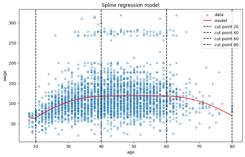
Voluntary exercise 2: Dynamic plotting#
You might have noticed that sometimes it is hard to see the cutpoints, especially when two bins share very similar estimates (see ). Therefore, it makes sense to highlight the cut points somehow when plotting the models.
Grab a model of your choice and modify the code so that the cut points are marked by black, dashed, vertical lines.
Try to make your code dynamic, meaning it dynamically accepts cut points provided in the
cut_pointslist and automatically fits and plots the model accordingly.Add a legend to the plot and label all lines and and data.
cut_points = (20,40,60,80)

# Fit the model with custom knots
transformed_age = patsy.dmatrix(f"bs(age, knots={str(cut_points)}, degree=2)",
                                data={"age": df['age']},
                                return_type='dataframe')

model = sm.OLS(df['wage'], transformed_age)
model_fit = model.fit()

# Plot the model
plt.figure(figsize=(10, 6))
xp = np.linspace(df['age'].min(), df['age'].max(), 100)
xp_trans = patsy.dmatrix("bs(xp, knots=(20,40,60,80), degree=2)",
                         data={"xp": xp},
                         return_type='dataframe')

predictions = model_fit.predict(xp_trans)

sns.scatterplot(data=df, x="age", y="wage", alpha=0.4, label="data")
plt.plot(xp, predictions, color='red', label="model")
plt.title("Spline regression model");

for cut in cut_points:
    plt.axvline(cut, color='black', linestyle='--', label=f"cut point {cut}")

plt.legend();