Logistic Regression#
Exercise 1: Loading the Data#
For today’s exercise we will use the Breast Cancer Wisconsin (Diagnostic). It is a collection of data used for predicting whether a breast tumor is malignant (cancerous) or benign (non-cancerous), containinh information derived from images of breast mass samples obtained through fine needle aspirates.
The dataset consists of 569 samples with 30 features that measure various characteristics of cell nuclei, such as radius, texture, perimeter, and area. Each sample is labeled as either malignant (1) or benign (0).
Please visit the documentation and familiarize yourself with the dataset.
Take an initial look at the features (predictors) and targets (outcomes) through the
.head()method.
import pandas as pd
import numpy as np
import matplotlib.pyplot as plt
from sklearn.linear_model import LogisticRegression
from sklearn.metrics import classification_report, confusion_matrix
from ucimlrepo import fetch_ucirepo

# Fetch dataset
breast_cancer_wisconsin_diagnostic = fetch_ucirepo(id=17)

# Data (as pandas dataframes)
X = breast_cancer_wisconsin_diagnostic.data.features
y = breast_cancer_wisconsin_diagnostic.data.targets

# Convert y to a 1D array (this is the required input for the logistic regression model)
y = np.ravel(y)

# Print information
print(breast_cancer_wisconsin_diagnostic.variables)
print(X.head())
print(y)
                  name     role         type demographic description units  \
0                   ID       ID  Categorical        None        None  None
1            Diagnosis   Target  Categorical        None        None  None
2              radius1  Feature   Continuous        None        None  None
3             texture1  Feature   Continuous        None        None  None
4           perimeter1  Feature   Continuous        None        None  None
5                area1  Feature   Continuous        None        None  None
6          smoothness1  Feature   Continuous        None        None  None
7         compactness1  Feature   Continuous        None        None  None
8           concavity1  Feature   Continuous        None        None  None
9      concave_points1  Feature   Continuous        None        None  None
10           symmetry1  Feature   Continuous        None        None  None
11  fractal_dimension1  Feature   Continuous        None        None  None
12             radius2  Feature   Continuous        None        None  None
13            texture2  Feature   Continuous        None        None  None
14          perimeter2  Feature   Continuous        None        None  None
15               area2  Feature   Continuous        None        None  None
16         smoothness2  Feature   Continuous        None        None  None
17        compactness2  Feature   Continuous        None        None  None
18          concavity2  Feature   Continuous        None        None  None
19     concave_points2  Feature   Continuous        None        None  None
20           symmetry2  Feature   Continuous        None        None  None
21  fractal_dimension2  Feature   Continuous        None        None  None
22             radius3  Feature   Continuous        None        None  None
23            texture3  Feature   Continuous        None        None  None
24          perimeter3  Feature   Continuous        None        None  None
25               area3  Feature   Continuous        None        None  None
26         smoothness3  Feature   Continuous        None        None  None
27        compactness3  Feature   Continuous        None        None  None
28          concavity3  Feature   Continuous        None        None  None
29     concave_points3  Feature   Continuous        None        None  None
30           symmetry3  Feature   Continuous        None        None  None
31  fractal_dimension3  Feature   Continuous        None        None  None

   missing_values
0              no
1              no
2              no
3              no
4              no
5              no
6              no
7              no
8              no
9              no
10             no
11             no
12             no
13             no
14             no
15             no
16             no
17             no
18             no
19             no
20             no
21             no
22             no
23             no
24             no
25             no
26             no
27             no
28             no
29             no
30             no
31             no
   radius1  texture1  perimeter1   area1  smoothness1  compactness1  \
0    17.99     10.38      122.80  1001.0      0.11840       0.27760
1    20.57     17.77      132.90  1326.0      0.08474       0.07864
2    19.69     21.25      130.00  1203.0      0.10960       0.15990
3    11.42     20.38       77.58   386.1      0.14250       0.28390
4    20.29     14.34      135.10  1297.0      0.10030       0.13280

   concavity1  concave_points1  symmetry1  fractal_dimension1  ...  radius3  \
0      0.3001          0.14710     0.2419             0.07871  ...    25.38
1      0.0869          0.07017     0.1812             0.05667  ...    24.99
2      0.1974          0.12790     0.2069             0.05999  ...    23.57
3      0.2414          0.10520     0.2597             0.09744  ...    14.91
4      0.1980          0.10430     0.1809             0.05883  ...    22.54

   texture3  perimeter3   area3  smoothness3  compactness3  concavity3  \
0     17.33      184.60  2019.0       0.1622        0.6656      0.7119
1     23.41      158.80  1956.0       0.1238        0.1866      0.2416
2     25.53      152.50  1709.0       0.1444        0.4245      0.4504
3     26.50       98.87   567.7       0.2098        0.8663      0.6869
4     16.67      152.20  1575.0       0.1374        0.2050      0.4000

   concave_points3  symmetry3  fractal_dimension3
0           0.2654     0.4601             0.11890
1           0.1860     0.2750             0.08902
2           0.2430     0.3613             0.08758
3           0.2575     0.6638             0.17300
4           0.1625     0.2364             0.07678

[5 rows x 30 columns]
['M' 'M' 'M' 'M' 'M' 'M' 'M' 'M' 'M' 'M' 'M' 'M' 'M' 'M' 'M' 'M' 'M' 'M'
 'M' 'B' 'B' 'B' 'M' 'M' 'M' 'M' 'M' 'M' 'M' 'M' 'M' 'M' 'M' 'M' 'M' 'M'
 'M' 'B' 'M' 'M' 'M' 'M' 'M' 'M' 'M' 'M' 'B' 'M' 'B' 'B' 'B' 'B' 'B' 'M'
 'M' 'B' 'M' 'M' 'B' 'B' 'B' 'B' 'M' 'B' 'M' 'M' 'B' 'B' 'B' 'B' 'M' 'B'
 'M' 'M' 'B' 'M' 'B' 'M' 'M' 'B' 'B' 'B' 'M' 'M' 'B' 'M' 'M' 'M' 'B' 'B'
 'B' 'M' 'B' 'B' 'M' 'M' 'B' 'B' 'B' 'M' 'M' 'B' 'B' 'B' 'B' 'M' 'B' 'B'
 'M' 'B' 'B' 'B' 'B' 'B' 'B' 'B' 'B' 'M' 'M' 'M' 'B' 'M' 'M' 'B' 'B' 'B'
 'M' 'M' 'B' 'M' 'B' 'M' 'M' 'B' 'M' 'M' 'B' 'B' 'M' 'B' 'B' 'M' 'B' 'B'
 'B' 'B' 'M' 'B' 'B' 'B' 'B' 'B' 'B' 'B' 'B' 'B' 'M' 'B' 'B' 'B' 'B' 'M'
 'M' 'B' 'M' 'B' 'B' 'M' 'M' 'B' 'B' 'M' 'M' 'B' 'B' 'B' 'B' 'M' 'B' 'B'
 'M' 'M' 'M' 'B' 'M' 'B' 'M' 'B' 'B' 'B' 'M' 'B' 'B' 'M' 'M' 'B' 'M' 'M'
 'M' 'M' 'B' 'M' 'M' 'M' 'B' 'M' 'B' 'M' 'B' 'B' 'M' 'B' 'M' 'M' 'M' 'M'
 'B' 'B' 'M' 'M' 'B' 'B' 'B' 'M' 'B' 'B' 'B' 'B' 'B' 'M' 'M' 'B' 'B' 'M'
 'B' 'B' 'M' 'M' 'B' 'M' 'B' 'B' 'B' 'B' 'M' 'B' 'B' 'B' 'B' 'B' 'M' 'B'
 'M' 'M' 'M' 'M' 'M' 'M' 'M' 'M' 'M' 'M' 'M' 'M' 'M' 'M' 'B' 'B' 'B' 'B'
 'B' 'B' 'M' 'B' 'M' 'B' 'B' 'M' 'B' 'B' 'M' 'B' 'M' 'M' 'B' 'B' 'B' 'B'
 'B' 'B' 'B' 'B' 'B' 'B' 'B' 'B' 'B' 'M' 'B' 'B' 'M' 'B' 'M' 'B' 'B' 'B'
 'B' 'B' 'B' 'B' 'B' 'B' 'B' 'B' 'B' 'B' 'B' 'M' 'B' 'B' 'B' 'M' 'B' 'M'
 'B' 'B' 'B' 'B' 'M' 'M' 'M' 'B' 'B' 'B' 'B' 'M' 'B' 'M' 'B' 'M' 'B' 'B'
 'B' 'M' 'B' 'B' 'B' 'B' 'B' 'B' 'B' 'M' 'M' 'M' 'B' 'B' 'B' 'B' 'B' 'B'
 'B' 'B' 'B' 'B' 'B' 'M' 'M' 'B' 'M' 'M' 'M' 'B' 'M' 'M' 'B' 'B' 'B' 'B'
 'B' 'M' 'B' 'B' 'B' 'B' 'B' 'M' 'B' 'B' 'B' 'M' 'B' 'B' 'M' 'M' 'B' 'B'
 'B' 'B' 'B' 'B' 'M' 'B' 'B' 'B' 'B' 'B' 'B' 'B' 'M' 'B' 'B' 'B' 'B' 'B'
 'M' 'B' 'B' 'M' 'B' 'B' 'B' 'B' 'B' 'B' 'B' 'B' 'B' 'B' 'B' 'B' 'M' 'B'
 'M' 'M' 'B' 'M' 'B' 'B' 'B' 'B' 'B' 'M' 'B' 'B' 'M' 'B' 'M' 'B' 'B' 'M'
 'B' 'M' 'B' 'B' 'B' 'B' 'B' 'B' 'B' 'B' 'M' 'M' 'B' 'B' 'B' 'B' 'B' 'B'
 'M' 'B' 'B' 'B' 'B' 'B' 'B' 'B' 'B' 'B' 'B' 'M' 'B' 'B' 'B' 'B' 'B' 'B'
 'B' 'M' 'B' 'M' 'B' 'B' 'M' 'B' 'B' 'B' 'B' 'B' 'M' 'M' 'B' 'M' 'B' 'M'
 'B' 'B' 'B' 'B' 'B' 'M' 'B' 'B' 'M' 'B' 'M' 'B' 'M' 'M' 'B' 'B' 'B' 'M'
 'B' 'B' 'B' 'B' 'B' 'B' 'B' 'B' 'B' 'B' 'B' 'M' 'B' 'M' 'M' 'B' 'B' 'B'
 'B' 'B' 'B' 'B' 'B' 'B' 'B' 'B' 'B' 'B' 'B' 'B' 'B' 'B' 'B' 'B' 'B' 'B'
 'B' 'B' 'B' 'B' 'M' 'M' 'M' 'M' 'M' 'M' 'B']
Exercise 2: Fitting the prediction model#
Fit a logitic regression model using all predictors for predicting
Get and print the accuracy of the model.
Get and print the confusion matrix for the target variable.
Review the classification report and interpret the results.
Hint: If you get a warning about convergence, try setting max_iter=10000 in the logistic regression class.
model = LogisticRegression(max_iter=10000)
results = model.fit(X, y)

# Get the intercept and coefficients
intercept = results.intercept_
coef = results.coef_

print("Intercept:", intercept)
print("Coefficients:", coef)

# Evaluate the model using predictions
print("Model accuracy:", model.score(X, y))

# Confusion Matrix
conf = confusion_matrix(y, model.predict(X))
print("Confusion matrix:\n", conf)

#classification report
from sklearn.metrics import classification_report
report = classification_report(y, model.predict(X))
print(report)
Intercept: [-27.95056684]
Coefficients: [[-1.01649102 -0.1801684   0.27565655 -0.0226662   0.1788688   0.22074883
   0.53685545  0.29603555  0.26639959  0.03046789  0.07816283 -1.25532588
  -0.11582457  0.10854792  0.02539334 -0.06767259  0.03651147  0.03822884
   0.03627027 -0.0140333  -0.15086497  0.43624862  0.10562901  0.01380557
   0.35772193  0.68749004  1.4271106   0.60399598  0.72848145  0.09506939]]
Model accuracy: 0.9578207381370826
Confusion matrix:
 [[348   9]
 [ 15 197]]
              precision    recall  f1-score   support

           B       0.96      0.97      0.97       357
           M       0.96      0.93      0.94       212

    accuracy                           0.96       569
   macro avg       0.96      0.95      0.95       569
weighted avg       0.96      0.96      0.96       569
Voluntary exercise#
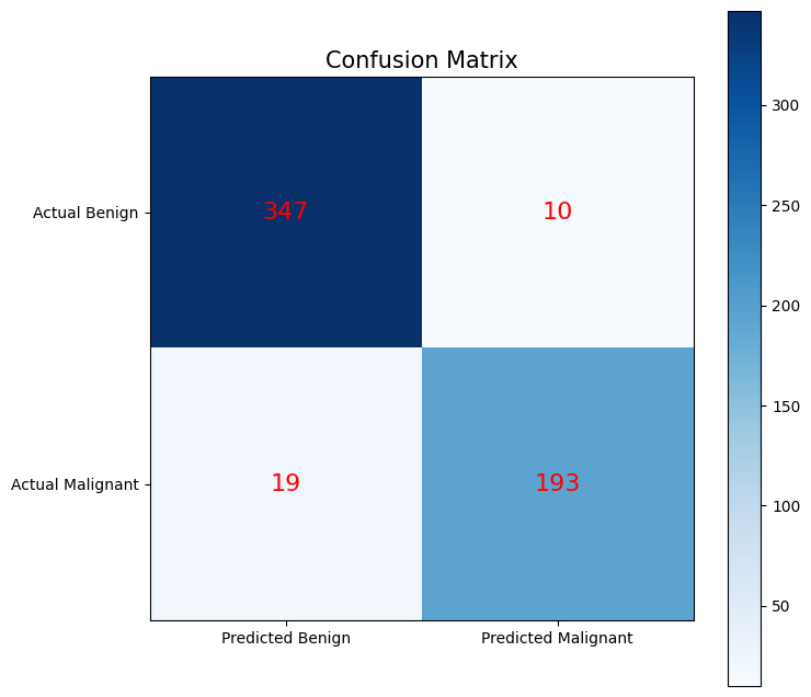
Try to create a custom plot which visualizes the confusion matrix It should contain:
The four squares of the matrix (color coded)
Labels of the actual values in the middle of each square
Labels for all squares
A colorbar
A title
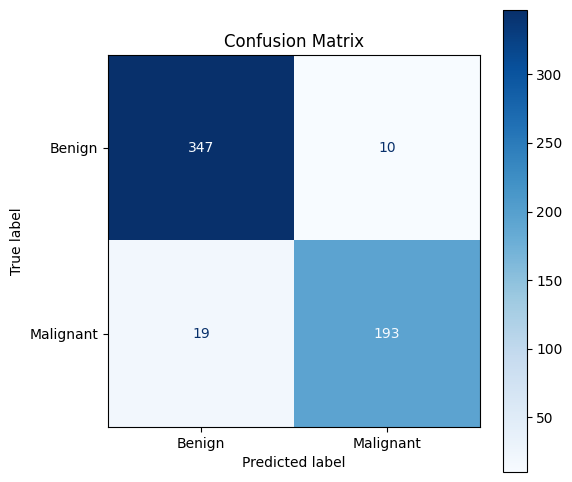
Use
ConfusionMatrixDisplay()from scikit-learn to achieve the same goal (and see that sometimes it makes sense to not re-invent the wheel :))
# 1. Plot a custom confusion matrix
fig, ax = plt.subplots(figsize=(8, 8))
cax = ax.imshow(conf, cmap='Blues')

# labels
ax.xaxis.set(ticks=(0, 1), ticklabels=('Predicted Benign', 'Predicted Malignant'))
ax.yaxis.set(ticks=(0, 1), ticklabels=('Actual Benign', 'Actual Malignant'))

# Annotate the confusion matrix
for i in range(2):
    for j in range(2):
        ax.text(j, i, conf[i, j], ha='center', va='center', color='red', fontsize=16)

ax.set_title('Confusion Matrix', fontsize=15)

plt.colorbar(cax)
plt.show()

# 2. Using scikit-learn
from sklearn.metrics import ConfusionMatrixDisplay

# Display the confusion matrix using scikit-learn
fig, ax = plt.subplots(figsize=(6, 6))
disp = ConfusionMatrixDisplay(confusion_matrix=conf,
                              display_labels=["Benign", "Malignant"])

disp.plot(cmap='Blues', ax=ax, colorbar=True)
plt.title("Confusion Matrix")
plt.show()