12.1 Polynomial Regression#
In many real-world situations, the relationship between a predictor and an outcome is not strictly linear. As a motivating example, consider predicting an exam grade (0–100%) from the number of hours a student studied. While studying more may initially improve performance, studying long hours can lead to fatigue or burnout, ultimately reducing performance. A pattern, which a simple linear regression would fail to find.
Polynomial regression extends linear regression by including higher-order terms of a predictor variable. This allows us to model curved relationships while still using the familiar linear regression framework.
To demonstrate this idea, we will simulate a dataset with two variables:
study_time: hours studiedgrade: exam grade in percent
   study_time     grades
0    5.851239  55.986343
1   12.517880  77.156030
2    6.553283  56.543544
3   12.262320  78.000597
4    9.297537  66.754832
As always, it is good practice to visualise the data before fitting any model:
import seaborn as sns
import matplotlib.pyplot as plt

fig, ax = plt.subplots(figsize=(8,5))
sns.scatterplot(data=df, x="study_time", y="grades", alpha=0.6, ax=ax)
ax.set(xlabel="Study time [h]", ylabel="Grade [%]", title="Study-time vs. Grade");
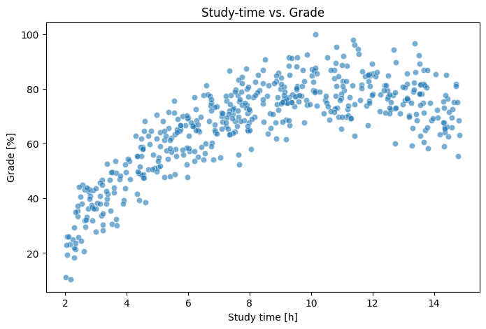
The plot clearly suggests a non-linear relationship: grades increase with study time up to a point until they level out (or maybe even slightly start to decline).
Fitting polynomial models#
In a standard linear regression with one predictor, our model has the form:
However, this assumes a linear relationship between \(x\) (e.g., study time) and \(y\) (e.g., grades). If we suspect a non-linear relationship, we can augment our single feature \(x\) with additional powers of \(x\) (e.g., \(x^2, x^3, \dots\)). This creates a polynomial model, for instance:
We will now fit two models to the data:
A linear regression model (first-order polynomial)
A quadratic regression model (second-order polynomial)
Both models are fitted using ordinary least squares (OLS). The key idea is that we transform the predictor variable into polynomial features and then apply a standard linear regression model.
First order polynomial#
To create the feature matrix, we use PolynomialFeatures from sciki-learn:
from sklearn.preprocessing import PolynomialFeatures

polynomial_features_p1 = PolynomialFeatures(degree=1, include_bias=True)
study_time_p1 = polynomial_features_p1.fit_transform(study_time.reshape(-1, 1))
But what are polynomial features?
OLS regression fits linear relationships between predictors (features) and the outcome. To fit a polynomial, we thus need to transform each original feature into “polynomial features” (e.g., instead of only \(x\) we also add \(x^2, x^3, \ldots\)) and then feed these new features into the linear regression model. This means, although the regression is still linear in its parameters, the relationship between the original predictor(s) \(X\) and the outcome \(y\) can be non-linear once polynomial terms are included.
Creating the polynomial feature matrix
When using PolynomialFeatures(degree=1, include_bias=True), degree=1 means we want to create polynomial features up to (and including) the first order. include_bias=True means a column of all 1’s (the “bias term”) should be added, corresponding to the intercept \(\beta_0\).
For a first-order polynomial, this is then simply a matrix which contains the intercept and the original feature \(x\):
In scikit-learn, this transformation can be performed with .fit_transform(study_time.reshape(-1, 1)) which does two things:
It reshapes
study_timefrom shape(n,)into a 2D array of shape(n,1)by using.reshape(-1, 1). This is the expected input for the sklearn library, as it would add columns along the scond dimension for higher orders.It applies the transformation to the original data, producing a 2D array of shape
n, 2(fordegree=1), where \(n\) is the number of data points. The first column ofstudy_time_p1is all 1’s (intercept), and the second column is the original study times becausedegree=1is the same as a standard linear regression. However, if you later decide to use higher degrees, you will get columns for \(x^1,x^2, \dots x^n\). That’s when you can capture curved relationships in your model.
With the features created, we can then use the standard sm.OLS() approach to create and fit the model:
import statsmodels.api as sm

model_linear = sm.OLS(grades, study_time_p1)
model_linear_fit = model_linear.fit()
We can then get the model predictions and residuals:
x_predict = np.linspace(df["study_time"].min(), df["study_time"].max(), 500)
x_predict_p1 = polynomial_features_p1.transform(x_predict.reshape(-1, 1))

linear_predictions = model_linear_fit.predict(x_predict_p1)
linear_residuals = model_linear_fit.resid
And plot them:
fig, ax = plt.subplots(1, 2, figsize=(8,4))

sns.scatterplot(data=df, x="study_time", y="grades", color='blue', alpha=0.5, ax=ax[0])
ax[0].plot(x_predict, linear_predictions, color='red', linewidth=2)
ax[0].set(title='Linear Regression')

sns.scatterplot(data=df, x="study_time", y=linear_residuals, color='red', alpha=0.5, ax=ax[1])
ax[1].axhline(0, linestyle='--')
ax[1].set(title="Residuals", ylim=(-55, 55));
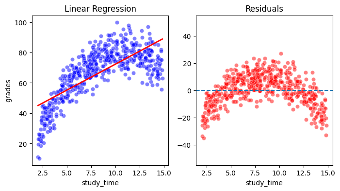
From the upper plot one can already see that while there is a clear linear trend present in the data, the first order model can not fully capture the non-linear relationship. This becomes even more clear if you look at the residuals, which have the positive linear trend removed. You can easily see that the residuals are systematically related to the value of \(x\), which is a graphical diagnosis for the existence of a non-linear relationship, higher than degree 1.
Second order polynomial#
We will now fit a second-order polynomial model to improve on the previous one. The procedure is the same as before, except we now use degree=2 for our features. This will create a feature matrix which looks like this:
polynomial_features_p2 = PolynomialFeatures(degree=2, include_bias=True)
study_time_p2 = polynomial_features_p2.fit_transform(study_time.reshape(-1, 1))

model_quadratic = sm.OLS(grades, study_time_p2)
model_quadratic_fit = model_quadratic.fit()
x_predict = np.linspace(df["study_time"].min(), df["study_time"].max(), 500)
x_predict_p2 = polynomial_features_p2.transform(x_predict.reshape(-1, 1))

quadratic_predictions = model_quadratic_fit.predict(x_predict_p2)
quadratic_residuals = model_quadratic_fit.resid
fig, ax = plt.subplots(1, 2, figsize=(8,4))

sns.scatterplot(data=df, x="study_time", y="grades", color='blue', alpha=0.5, ax=ax[0])
ax[0].plot(x_predict, quadratic_predictions, color='red', linewidth=2)
ax[0].set(title='Quadratic Regression')

sns.scatterplot(data=df, x="study_time", y=quadratic_residuals, color='red', alpha=0.5, ax=ax[1])
ax[1].axhline(0, linestyle='--')
ax[1].set(title="Residuals", ylim=(-55, 55));
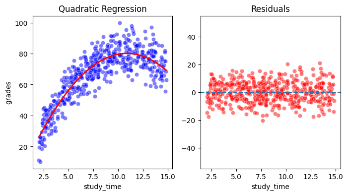
You can see that the model fits the data much better. Also, the residuals are now much smaller and do not show any systematic pattern (only the noise remains), which means we were succesful in capturing the non-linear relationship in the data.
Interpretation#
The interpretation of the model results is similar to that for normal linear models, except that we now have estimates for higher-order terms as well:
print(model_quadratic_fit.summary())
                            OLS Regression Results
==============================================================================
Dep. Variable:                      y   R-squared:                       0.802
Model:                            OLS   Adj. R-squared:                  0.801
Method:                 Least Squares   F-statistic:                     1007.
Date:                Wed, 28 Jan 2026   Prob (F-statistic):          1.50e-175
Time:                        10:57:55   Log-Likelihood:                -1714.2
No. Observations:                 500   AIC:                             3434.
Df Residuals:                     497   BIC:                             3447.
Df Model:                           2
Covariance Type:            nonrobust
==============================================================================
                 coef    std err          t      P>|t|      [0.025      0.975]
------------------------------------------------------------------------------
const         -1.3650      1.763     -0.774      0.439      -4.828       2.098
x1            14.9837      0.463     32.353      0.000      14.074      15.894
x2            -0.6888      0.027    -25.493      0.000      -0.742      -0.636
==============================================================================
Omnibus:                        2.570   Durbin-Watson:                   2.050
Prob(Omnibus):                  0.277   Jarque-Bera (JB):                2.125
Skew:                          -0.007   Prob(JB):                        0.346
Kurtosis:                       2.681   Cond. No.                         560.
==============================================================================

Notes:
[1] Standard Errors assume that the covariance matrix of the errors is correctly specified.
Coefficients
Intercept (
const)
Not statistically significant. The intercept represents the predicted grade at zero hours of study. However, as the minimum hours of study in our data is 2, this might not be a meaningful estimate. We will change this with centering in the next section.Linear term (
x1)
Positive and highly significant. This indicates that grades initially increase as study time increases.Quadratic term (
x2)
Negative and highly significant. This means the model predicts an initial increase in grade as study time increases, followed by a decrease past a certain point.
Model Fit
R-squared = 0.802: 80% of the variance ingradeis explained.If we compare this to the linear model, we see that the quadratic model explains much more variance (80% vs. 54%) and provides a better fit according to AIC/BIC:
print(model_linear_fit.summary())
                            OLS Regression Results
==============================================================================
Dep. Variable:                      y   R-squared:                       0.543
Model:                            OLS   Adj. R-squared:                  0.542
Method:                 Least Squares   F-statistic:                     592.4
Date:                Wed, 28 Jan 2026   Prob (F-statistic):           8.63e-87
Time:                        10:57:55   Log-Likelihood:                -1923.2
No. Observations:                 500   AIC:                             3850.
Df Residuals:                     498   BIC:                             3859.
Df Model:                           1
Covariance Type:            nonrobust
==============================================================================
                 coef    std err          t      P>|t|      [0.025      0.975]
------------------------------------------------------------------------------
const         38.1848      1.270     30.072      0.000      35.690      40.680
x1             3.4150      0.140     24.339      0.000       3.139       3.691
==============================================================================
Omnibus:                       13.789   Durbin-Watson:                   1.964
Prob(Omnibus):                  0.001   Jarque-Bera (JB):               14.517
Skew:                          -0.409   Prob(JB):                     0.000704
Kurtosis:                       2.837   Cond. No.                         22.9
==============================================================================

Notes:
[1] Standard Errors assume that the covariance matrix of the errors is correctly specified.