Exploratory Factor Analysis#
Exercise 1: The Dataset#
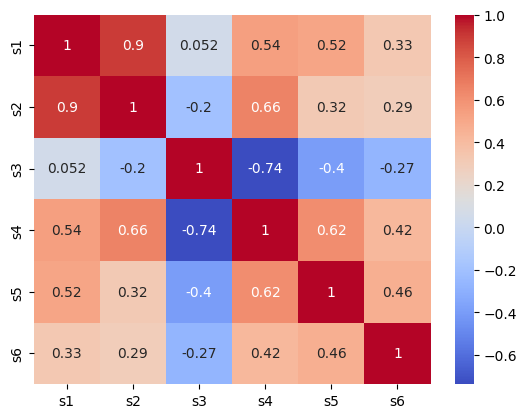
Remember the diabetes dataset which we used in a few weeks ago to predict the presence of diabetes. This week, our goal will be to explore the six blood serum measures, aiming to find underlying factors within them.
The data is already loaded and processed. Please do the following:
Print and read through the description of the dataset using the
.DESCRattributeInspect the DataFrame and check if it contains the correct variables
Plot the correlation matrix of the blood serum measures (e.g. with
sns.heatmap()orplt.imshow()).
import pandas as pd
import seaborn as sns
import matplotlib.pyplot as plt
from sklearn import datasets

# Load the six blood serum measures (s1-s6) of the diabetes dataset
diabetes_data = datasets.load_diabetes(as_frame=True)
df = diabetes_data.data[['s1', 's2', 's3', 's4', 's5', 's6']]

print(diabetes_data.DESCR)
print(df.head())
sns.heatmap(df.corr(), cmap='coolwarm', annot=True);
.. _diabetes_dataset:

Diabetes dataset
----------------

Ten baseline variables, age, sex, body mass index, average blood
pressure, and six blood serum measurements were obtained for each of n =
442 diabetes patients, as well as the response of interest, a
quantitative measure of disease progression one year after baseline.

**Data Set Characteristics:**

:Number of Instances: 442

:Number of Attributes: First 10 columns are numeric predictive values

:Target: Column 11 is a quantitative measure of disease progression one year after baseline

:Attribute Information:
    - age     age in years
    - sex
    - bmi     body mass index
    - bp      average blood pressure
    - s1      tc, total serum cholesterol
    - s2      ldl, low-density lipoproteins
    - s3      hdl, high-density lipoproteins
    - s4      tch, total cholesterol / HDL
    - s5      ltg, possibly log of serum triglycerides level
    - s6      glu, blood sugar level

Note: Each of these 10 feature variables have been mean centered and scaled by the standard deviation times the square root of `n_samples` (i.e. the sum of squares of each column totals 1).

Source URL:
https://www4.stat.ncsu.edu/~boos/var.select/diabetes.html

For more information see:
Bradley Efron, Trevor Hastie, Iain Johnstone and Robert Tibshirani (2004) "Least Angle Regression," Annals of Statistics (with discussion), 407-499.
(https://web.stanford.edu/~hastie/Papers/LARS/LeastAngle_2002.pdf)

         s1        s2        s3        s4        s5        s6
0 -0.044223 -0.034821 -0.043401 -0.002592  0.019907 -0.017646
1 -0.008449 -0.019163  0.074412 -0.039493 -0.068332 -0.092204
2 -0.045599 -0.034194 -0.032356 -0.002592  0.002861 -0.025930
3  0.012191  0.024991 -0.036038  0.034309  0.022688 -0.009362
4  0.003935  0.015596  0.008142 -0.002592 -0.031988 -0.046641
Exercise 2: Fitting the Model#
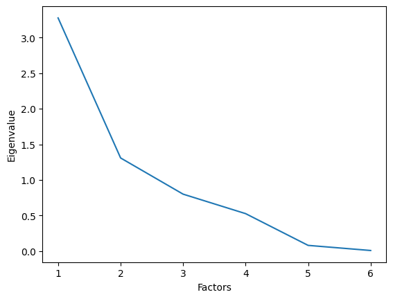
Use factor_analyzer package to fit a first non-rotated model with the minres optimizer and the number of factors corresponding to the number of items. Determine the most suitable number of factors using the Kaiser criterion.
from factor_analyzer import FactorAnalyzer

# Fit the initial model
fa = FactorAnalyzer(rotation=None, n_factors=6)
fa.fit(df)

# Determine the number of factors
ev, __ = fa.get_eigenvalues()
print(ev)

ax = sns.lineplot(x=range(1, len(ev) + 1), y=ev)
ax.set_xlabel("Factors")
ax.set_ylabel("Eigenvalue");
[3.27565985 1.30852971 0.80016549 0.52650327 0.08052117 0.00862051]
Exercise 3: Loadings & Communalities#
After selecting the number of factors, fit a final model with oblimin rotation. Print the rotated factor loadings and communalities. Do the communalities suggest a good model fit?
fa2 = FactorAnalyzer(n_factors=2, rotation='oblimin')
fa2.fit(df)

print("Loadings:\n", fa2.loadings_)
print("Communalities:", fa2.get_communalities())
Loadings:
 [[ 1.04095052 -0.06391605]
 [ 0.79721715  0.14763963]
 [ 0.23543195 -0.9377997 ]
 [ 0.36511127  0.81892308]
 [ 0.33348504  0.46899681]
 [ 0.24832244  0.34203792]]
Communalities: [1.08766324 0.65735264 0.93489647 0.80394125 0.33117028 0.17865398]
Voluntary exercise 1: Improving the Fit#
Look again at the Communalities. Some variables are badly represented by the factor structure. Exclude them and fit the model again. Did the fit improve?
# Exclude variables
df = df.drop(columns=['s5', 's6']) #s5 & s6 have low communalities, meaning they are not well represented by the factor structure

# Fit the model
fa3 = FactorAnalyzer(n_factors=2, rotation='oblimin')
fa3.fit(df)

# Get loadings
l = fa3.loadings_
print(l)

# Get communalities
c = fa3.get_communalities()
print(c)
[[ 1.017817    0.12752987]
 [ 0.89155588 -0.12630942]
 [ 0.13112868  1.01673845]
 [ 0.48566271 -0.70742639]]
[1.05221532 0.81082596 1.05095181 0.73632037]