Introduction

This first lecture is mainly a review of the concepts covered in Basic Statistics (taught in Bachelor programmes). Disclosure: I use advanced large language models to help me convert my slides into continuous text for the following chapters more quickly. Please note that the generated text has been thoroughly revised by me, and that the text has been generated solely on the basis of keywords entered from my lecture slides. Let’s start!

1.1 On the basic objective of uni-, bi- and multi-variate statistics

Univariate methods are used when our data contains only a single variable. Unlike their multivariate counterparts, univariate methods do not address relationships or causes between variables. Instead, they focus on describing the characteristics and patterns within that single variable. We can think of it as taking a magnifying glass to a particular aspect of our data. Examples of univariate methods include the one-sample \(z\)-test, which is used to compare a sample mean with a known population mean when the population variance is known, or the one-way table \(\chi^2\)‐test, which helps us understand the distribution of a categorical variable.

If we extend our view a little beyond single variables, we come to bivariate methods, which are used when our data involve two variables. These methods allow us to explore the relationships between these two variables, revealing possible associations and dependencies. For example, we might use an independent samples t-test to compare the mean scores on an outcome variable between two groups, or we might estimate bivariate correlations to quantify the strength and direction of the linear relationship between two quantitative variables. Other bivariate methods include one-factor analysis of variance, which examines differences in means between several groups, and simple linear regression, where we model the relationship between two variables with a straight line, using one as a predictor of the other.

Moving further into the realm of statistical analysis, we come to multivariate methods, the tools we use to unravel the complexities of data sets containing at least three variables, but usually more. These methods allow us to explore the intricate relationships, and possibly even causal associations, between multiple variables simultaneously. This is where we begin to unravel the multi-determinacy of human behaviour, experience and action, recognising that these phenomena are rarely shaped by a single factor, but rather by the interplay of multiple influences.

In summary, multivariate methods allow us to move beyond simple associations to a deeper understanding. They help us to identify the interference of third variables, showing how an apparently direct relationship between two variables may be influenced by another lurking in the background. They also help to identify redundant relationships, showing us when multiple variables may be measuring similar underlying constructs, and can even reveal hidden relationships that would remain unresolved if only two variables were considered at a time. In essence, multivariate methods provide a more complete and nuanced picture of the complex realities we seek to understand.

Have you ever asked yourself: What is the fundamental aim of statistical models?

Statistics is mainly about learning from data. We collect data through experiments, studies and observations, and then we use statistical methods to extract meaningful insights and knowledge from that data. It’s like asking, “What probabilistic model could have generated the data we observed?” To answer this question, we rely on statistical models, which serve as essential tools and conceptual foundations for quantitative reasoning. These models provide the framework for intelligently extracting information from data, allowing us to go beyond raw numbers to uncover the underlying patterns and phenomena that shape human cognition, emotion, experience, behaviour and health. In addition, multivariate statistical models allow us to formalise relationships between variables using mathematical equations.

And what is the general approach and procedure for the modelling process?

The modelling process generally follows a number of key steps. First, we select a suitable model from a set of potential candidates, choosing a family of models that seems appropriate for the data and the research question. Second, we estimate the unknown quantities of the model, its parameters, by fitting the model to the data. This step involves finding the parameter values that best capture the observed patterns in the data. Third, we compare the performance of our fitted model with alternative models to assess its appropriateness and to determine whether a different model might provide a better representation of the data. Why do we do this? To test hypotheses, make predictions, measure the confidence of conclusions, etc.

In conclusion, we can think of the modelling process as a lens through which we interpret the data, and as of a reasonable approximation of the stochastic process on which confirmatory inference “about the world” is based.

1.2 What is a model?

But what exactly is a model?

An analogy might help: In the physical world, we use models to represent complex objects or systems in a simplified way. Think of a model aeroplane that captures the shape and structure of a real aeroplane, but is small enough to hold in your hand. Similarly, a model of a biological cell may be much larger than the actual cell, but it still conveys the essential components and their relationships. Just as physical models provide a condensed description of real-world objects, statistical models provide a simplified representation of data. A statistical model is typically much simpler than the data it describes and aims to capture the underlying structure as succinctly as possible. In essence, a statistical model can be thought of as a theory of how the observed data came about. It’s a way of making sense of the patterns and relationships in the data by proposing an underlying process that could have produced them.

We aim to find the model that most efficiently and accurately summarizes the way in which the data were generated.

The basic structure of a statistical model

\(data = model + error\)

Importantly, when we build statistical models, we essentially divide (we say “decompose”) the data into two parts. The first part is the part we can explain with our model, which represents the values we expect the data to take based on our current knowledge summarized in the model. The second part is what we call the error, which reflects the mismatch between our model’s predictions and the actual observed data. It is important to remember that this error is not a fixed value within the model, but varies between different data points. We say that the error is a random variable.

Note that we can use the model to predict the value of the data:

Prediction

\(\widehat{data}_{i} = model_{i}\)

where \(i\) indicates the observations.

And once we have the prediction, we can compute the error for each observation:

Compute the error

\(error_{i} = data_{i} - \widehat{data}_{i}\)

1.3 Two modeling cultures

It is helpful to understand that there are two main approaches to modelling multivariate data: Although the boundaries between them are blurred, we can speak of traditional statistical modelling (our module psy111) and statistical learning (our module psy112).

Statistical modelling, which has its roots in mathematics and a history dating back to the 17th century, emphasises inference. This means that it focuses on understanding the relationships between variables and drawing conclusions about the underlying population. It often relies on making assumptions about the data and typically works with smaller data sets.

Statistical learning emerged in the 1990s from the fields of computer science and artificial intelligence. It prioritises prediction accuracy and can often handle very large data sets (“big data”) with fewer assumptions.

Importantly: While these two approaches have traditionally been distinct, the boundaries between them are becoming increasingly blurred. For our purposes, this distinction serves primarily as a helpful way of understanding the broader landscape of data modelling.

1.4 The linear function

Remember two key terms!

Dependent variable

This is the outcome variable that our model aims to explain (usually referred to as \(Y\), previously referred to as data).

Independent variable

This is a variable that we wish to use in order to explain the dependent variable (usually referred to as \(X\), the predictor or predictors). Note that in multivariate models, there are multiple independent variables (\(X_1, X_2, ..., X_j\)).

Remember a bivariate distribution of data!

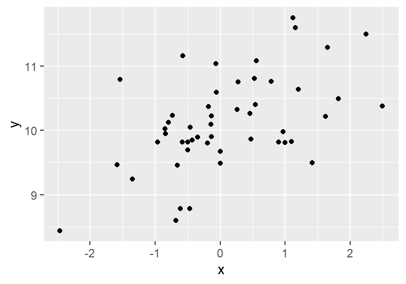
Fig. 7 Bivariate distribution of data points

When we work with a statistical model - for example, using a linear function as a model - we have several key objectives in mind. For example, we might want to

Describe the data: Imagine we are looking at the relationship between two variables, \(y\) and \(x\). Our model can help us describe how strong the linear relationship between them is. Are they closely related, or is the relationship weak?

Decide about parameters of a linear model: We can also use our model to make statistical decisions. For example, we might want to decide whether the relationship between \(y\) and \(x\) is statistically significant. Is the linear association pattern we observe real (population), or could it be due to chance (sampling \(N\) observations from the population)?

Make predictions about data cases: Perhaps the most important use of a statistical model to solve real life problems is to make predictions. If we know a certain value of \(x\) , our model can help us predict what the corresponding value of \(y\) is likely to be. This has applications in everything from predicting company sales to predicting patient outcomes.

A linear function is written as

\(y = a + b \cdot x \)

Independent variable

Note that the value of \(b\) indicates the slope of the straight line and **\(a\) **(intercept) indicates the value of \(y\) for \(x = 0\).

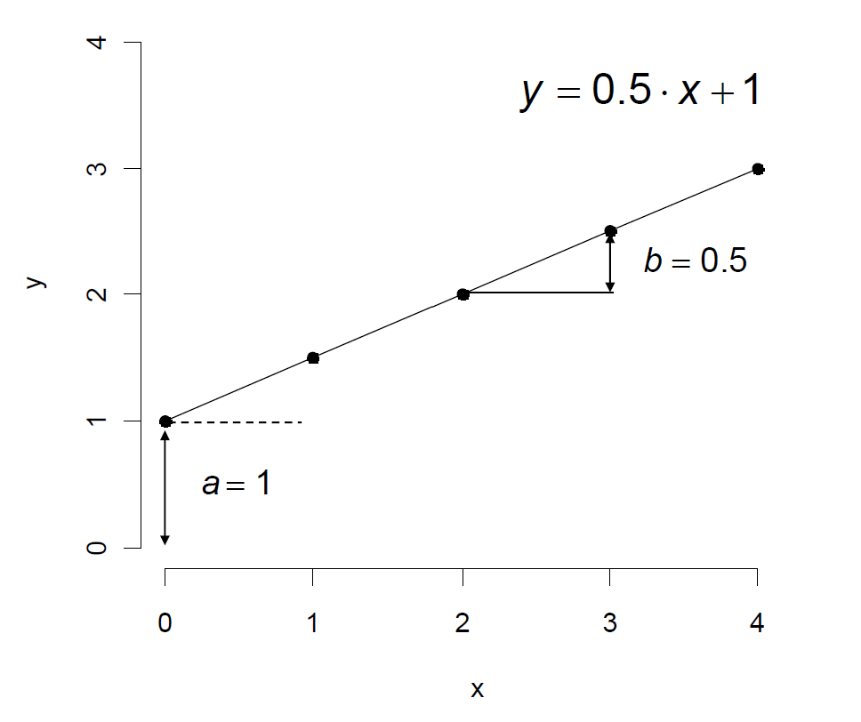
Fig. 8 The linear function

Interpretation of the intercept

The intercept indicates the expected value of \(y\) given \(x\) is zero.

Interpretation of the slope

The slope indicates the expected change of \(y\) given \(x\) changed in one unit.

Let’s take an empirical example. Suppose we measured the Conscientiousness (\(x\)) and Job Success (\(y\)) of three individuals. The following table and scatterplot show the observed scores in a two-dimensional space. Note that the index \(m\) indicates the cases. We also say observation units (here individuals).

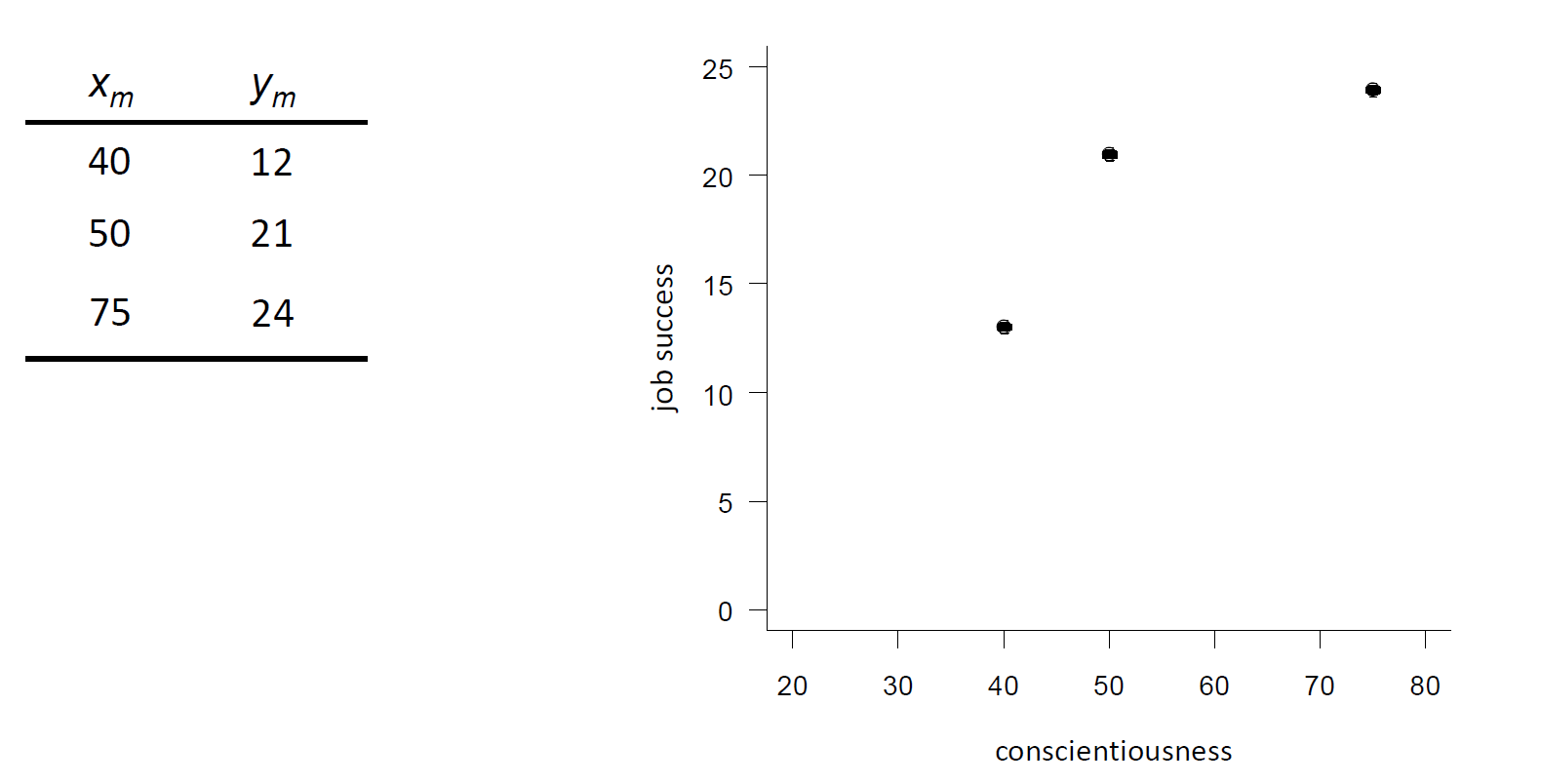
Fig. 9 Empirical example with scarce data

First, imagine that we only have data (= knowledge) on the Job Success of these three individuals. Someone would bring you a new case belonging to the same population (let’s say a fourth individual from the same company). What would be the best prediction you could make about this person’s Job Success, given your knowledge of the previous three people?