Multilevel Models#
The Dataset#
The Oxboys dataset consists of longitudinal height measurements for boys from Oxford, UK. Our goal for today is to predict height by age. The dataset contains the following variables:
Subject- Unique identifier for each child in the experimentage- The standardized ageheight- The height of the child in centimetersOccasion- The result of converting age from a continuous variable to a categorical one (can be ignored)
# Load packages
import numpy as np
import pandas as pd
import statsmodels.api as sm
import statsmodels.formula.api as smf
import seaborn as sns
import matplotlib.pyplot as plt

data = sm.datasets.get_rdataset("Oxboys", "nlme").data
data
| Subject | age | height | Occasion | |
|---|---|---|---|---|
| 0 | 1 | -1.0000 | 140.5 | 1 |
| 1 | 1 | -0.7479 | 143.4 | 2 |
| 2 | 1 | -0.4630 | 144.8 | 3 |
| 3 | 1 | -0.1643 | 147.1 | 4 |
| 4 | 1 | -0.0027 | 147.7 | 5 |
| ... | ... | ... | ... | ... |
| 229 | 26 | -0.0027 | 138.4 | 5 |
| 230 | 26 | 0.2466 | 138.9 | 6 |
| 231 | 26 | 0.5562 | 141.8 | 7 |
| 232 | 26 | 0.7781 | 142.6 | 8 |
| 233 | 26 | 1.0055 | 143.1 | 9 |
234 rows × 4 columns
Exercise 1: Data visualization#
To get a better feeling for the data, create two plots:
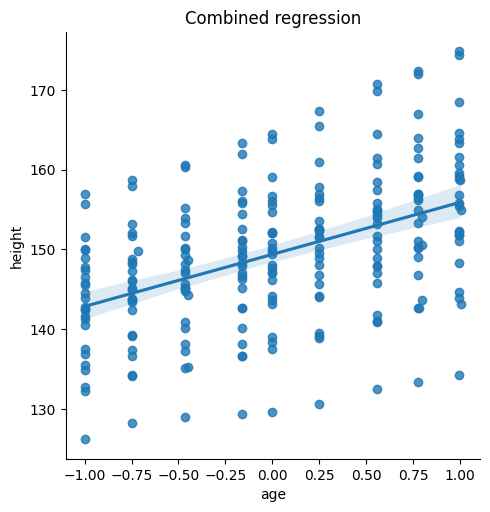
Plot 1: Scatterplot with a single regression line for
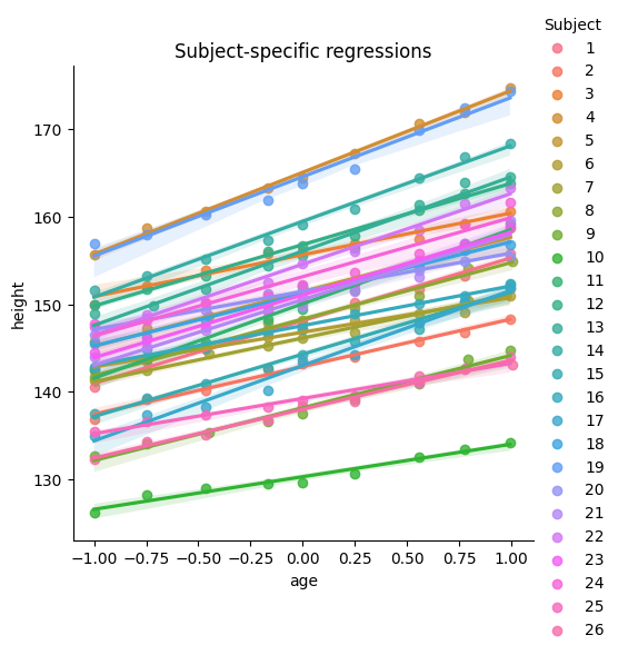
heightpredicted byagePlot 2: Scatterplot with a regression line for each subject for
heightpredicted byage.
Inspect the plots. Do you think multilevel modeling is needed for this data?
# Plot 1: Plot with single regression line for height predicted by age
sns.lmplot(x='age', y='height', data=data)
plt.title("Combined regression")

# Plot 2: Plot with a regressin line for each subject
sns.lmplot(x='age', y='height', hue='Subject', data=data)
plt.title("Subject-specific regressions");
Exercise 2: Fitting a null model#
To find out how much variance in height is explained by Subject we begin by fitting a null model without any predictors. Set up the model and inspect the model output. To further analyze the data, calculate the ICC and interpret it. Which model parameter indicates the amount of variance in the intercept?
# defining and fitting the model
model1 = smf.mixedlm("height ~ 1", data, groups=data["Subject"])
model1_fit = model1.fit(method="bfgs")

# print model summary
print(model1_fit.summary())

# Create ICC function for calculation
def calculate_icc(results):
    icc = results.cov_re / (results.cov_re + results.scale)

    return round(icc.values[0, 0], 4)
# calculate ICC
icc = calculate_icc(model1_fit)
print(f"The ICC is {icc}, meaning 74.45% of the variance in height is due to differences between subjects.")

# The `Group Var` row in the output show the variance of the intercept.
         Mixed Linear Model Regression Results
=======================================================
Model:            MixedLM Dependent Variable: height
No. Observations: 234     Method:             REML
No. Groups:       26      Scale:              21.7271
Min. group size:  9       Log-Likelihood:     -733.2949
Max. group size:  9       Converged:          Yes
Mean group size:  9.0
-------------------------------------------------------
           Coef.  Std.Err.   z    P>|z|  [0.025  0.975]
-------------------------------------------------------
Intercept 149.519    1.590 94.039 0.000 146.403 152.636
Group Var  63.314    4.221
=======================================================

The ICC is 0.7445, meaning 74.45% of the variance in height is due to differences between subjects.
Exercise 3: Fitting a random intercept model#
As seen in the null model, there is a lot of variance explained by the grouping variable Subject. Therefore, fitting one regression over all datapoints may lead to wrong interpretations and we need the model to account for inter-individual differences. To do so, please fit a random intercept model, predicting height with age. What is the average relationship between age and height?
model2 = smf.mixedlm("height ~ age", data, groups=data["Subject"])
model2_fit = model2.fit(method="bfgs")

print(model2_fit.summary())

# The average relationship between age and height is 6.524. For a one-unit increase in age, height is expected to increase by 6.524 units on average
         Mixed Linear Model Regression Results
=======================================================
Model:            MixedLM Dependent Variable: height
No. Observations: 234     Method:             REML
No. Groups:       26      Scale:              1.7181
Min. group size:  9       Log-Likelihood:     -470.0148
Max. group size:  9       Converged:          Yes
Mean group size:  9.0
-------------------------------------------------------
           Coef.  Std.Err.   z    P>|z|  [0.025  0.975]
-------------------------------------------------------
Intercept 149.372    1.590 93.934 0.000 146.255 152.488
age         6.524    0.133 49.228 0.000   6.264   6.784
Group Var  65.554   15.019
=======================================================
Exercise 4: Fitting a random intercept & random slope model#
To increase the flexibility in our model, we will now add random slopes as well, meaning that for every subject a random intecept and a random slope is fitted. Please specify the model and interpret the output.
model3 = smf.mixedlm("height ~ age", data, groups=data["Subject"], re_formula="~age")
model3_fit = model3.fit(method="bfgs")

print(model3_fit.summary())

# The slope variance is 2.825, suggesting there is considerable variability in how height changes with age across subjects.
# The correlation between slope and intercept is 0.105, meaning subjects with a larger intercept tend to have a more positive/steeper slope.
            Mixed Linear Model Regression Results
=============================================================
Model:              MixedLM   Dependent Variable:   height
No. Observations:   234       Method:               REML
No. Groups:         26        Scale:                0.4355
Min. group size:    9         Log-Likelihood:       -362.0455
Max. group size:    9         Converged:            Yes
Mean group size:    9.0
-------------------------------------------------------------
                 Coef.  Std.Err.   z    P>|z|  [0.025  0.975]
-------------------------------------------------------------
Intercept       149.372    1.585 94.217 0.000 146.264 152.479
age               6.525    0.336 19.404 0.000   5.866   7.185
Group Var        65.303   29.873
Group x age Cov   8.710    5.151
age Var           2.825    1.344
=============================================================
Voluntary exercise 1: Fitting a random slope & fixed intercept model#
Until now we either looked at random intercept - fixed slope models (only the intercepts vary accross subject) or at random intercept - random slope moddels (intercept and slope vary accross subects). However, it is also possible to fit fixed intercept & random slope models. Find out how to do it and specify such a model. What is different compared to the random intercept & random slope model?
Important information: There might be some warnings which refer to the model not converging. This is probably caused by the low variance in the slope (see above). The random effects in the model have very small or zero variance, indicating that the random effect might not be necessary or is poorly estimated. For now, you can ignore this warning. However, you should be extremely cautious when interpreting model estimates in case of convergence problems.
model4 = smf.mixedlm("height ~ age", data, groups=data["Subject"], re_formula="~age - 1")
model4_fit = model4.fit(method="bfgs")

print(model4_fit.summary())

# The is no estimate for the intercept variance. This is because we specified the intercept to be fixed.
# Consequently, there is also no estimate for the correlation between intercept and slope.
         Mixed Linear Model Regression Results
========================================================
Model:             MixedLM Dependent Variable: height
No. Observations:  234     Method:             REML
No. Groups:        26      Scale:              65.2748
Min. group size:   9       Log-Likelihood:     -819.0859
Max. group size:   9       Converged:          No
Mean group size:   9.0
--------------------------------------------------------
           Coef.  Std.Err.    z    P>|z|  [0.025  0.975]
--------------------------------------------------------
Intercept 149.372    0.528 282.643 0.000 148.336 150.408
age         6.521    0.822   7.934 0.000   4.910   8.132
age Var     0.216
========================================================
c:\Users\maku1542\Desktop\Main\Classes\psy11\.venv\Lib\site-packages\statsmodels\base\model.py:607: ConvergenceWarning: Maximum Likelihood optimization failed to converge. Check mle_retvals
  warnings.warn("Maximum Likelihood optimization failed to "
c:\Users\maku1542\Desktop\Main\Classes\psy11\.venv\Lib\site-packages\statsmodels\regression\mixed_linear_model.py:2206: ConvergenceWarning: MixedLM optimization failed, trying a different optimizer may help.
  warnings.warn(msg, ConvergenceWarning)
c:\Users\maku1542\Desktop\Main\Classes\psy11\.venv\Lib\site-packages\statsmodels\regression\mixed_linear_model.py:2218: ConvergenceWarning: Gradient optimization failed, |grad| = 4.108056
  warnings.warn(msg, ConvergenceWarning)
c:\Users\maku1542\Desktop\Main\Classes\psy11\.venv\Lib\site-packages\statsmodels\regression\mixed_linear_model.py:2261: ConvergenceWarning: The Hessian matrix at the estimated parameter values is not positive definite.
  warnings.warn(msg, ConvergenceWarning)